Solving Path of Exile item crafting with Reinforcement Learning
Background #
PoE (Path of Exile) is an ARPG similar to Diablo 2/3/4 or Last Epoch. You kill monsters, collect loot, and progress your character with increasingly better gear, which in turn allows you to complete more challenging content. PoE is somewhat infamous for its complexity. It was first released in 2013 and has received a large number of expansions, each adding new layers of mechanics to the game. Players with a thousand hours of playtime sometimes still call themselves beginners. One of PoE’s more complex systems is item crafting. Due to its high barrier of entry and risk of failure, many players choose to buy items from the trade market instead of crafting them. In this post, we will explore the question:
Given a target item, can we use an algorithm to learn the optimal sequence of actions to craft it?
We will look at a few approaches and eventually solve the problem with a model-based Reinforcement Learning algorithm.
Crafting in Path of Exile #
In PoE, many of the best items are not dropped by enemies. They are the result of a crafting process where players modify item attributes using various crafting currencies. But first let’s understand what items in PoE look like.
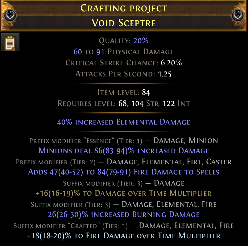
A sceptre with 2 prefixes and 3 suffixes
The above image is a Sceptre weapon in PoE. There are a lot of things going on, but we are mostly concerned with the modifiers such as 18% to Fire Damage Over Time Multiplier. The above item has 5 modifiers, listed at the bottom. There are 2 prefixes, and 3 suffixes. There is no fundamental difference between prefixes and suffixes except that they are different pools of possible modifiers. Some modifiers are always prefixes. Some are always suffixes.
A rare (yellow) item in PoE can have up to 6 modifiers with a maximum of 3 prefixes and 3 suffixes. A magic (blue) item can only have one prefix and one suffix. When PoE generates a rare item, e.g. dropped by an enemy, it does something like the following pseudocode:
item = Item("Void Sceptre", level=84)

# Spawn 4, 5, or 6 modifiers with 2/3, 1/4 or 1/12 probability
num_modifiers = np.random.choice([4, 5, 6], p=[2/3, 1/4, 1/12])

for _ in range(num_modifiers):
    # Get a list of spawnable modifiers and their probabilities
    # These depend on the item base type, level, and existing modifiers
    spawnable_modifiers, probs = get_spawnable_modifiers(item)
    # Sample a modifier
    modifier = np.random.choice(spawnable_modifiers, p=probs)
    # Add it to the item
    spawn_modifier(modifier)
In reality there are many additional checks and restrictions, but the basic idea is that modifiers are sampled from a distribution that depends on the current state of the item, including its base type, level, and existing modifiers. Luckily, people have extracted information to derive this distribution from game data and made it publicly available on websites such as craftofexile.com and poedb.tw. Each modifier has a weight associated with it, and its spawn probability is the normalized weight. For a Sceptre weapon the modifier data looks like this.
Crafting in PoE, at least to the extent that we are concerned with in this post, is the process of changing the modifiers on an item through various actions to achieve a desired outcome. These actions typically consist of applying currency to the item, or using other mechanics such as a crafting bench. Because the outcome of most actions is stochastic, crafts in PoE can consist of hundreds of steps, including looping certain actions until some condition is met before moving on to the next step. Let’s look at a basic example:
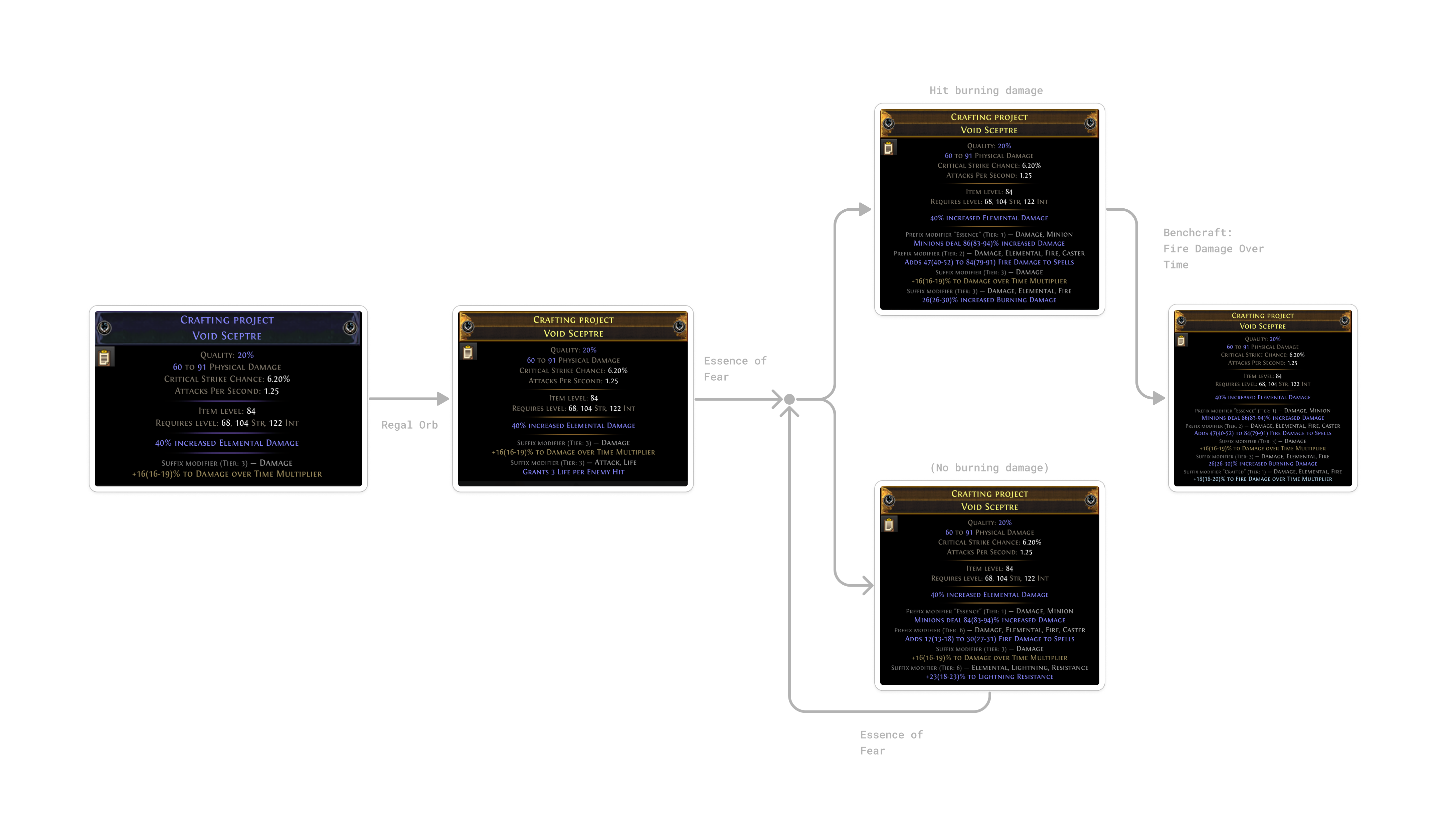
To craft the Void Sceptre we looked at above, we would follow these steps:
- Start with a Magic Sceptre with a fractured “Damage over time multiplier” modifier. A fractured modifier is fixed on the item and cannot be changed by subsequent actions.
- Use a Regal Orb to upgrade the item from a magic to a rare item. This will add a random modifier which we don’t care about since we will remove it later. We need to upgrade the item to a rare item so that we can use an Essence on it in the next step.
- Use a Essence of Fear to add a guaranteed “Increased Minion Damage” modifier while randomizing all other modifiers on the item, except for the fractured one. If the randomized modifiers include a desired modifier such as “Burning Damage”, continue to the next step. Otherwise, repeat this step.
- Use the crafting bench to add the “Fire Damage over Time multiplier” modifier to the item.
I picked this simple example for demonstration purposes, but many crafts in PoE are significantly more complex. There exist hundreds of different actions, many of which can be composed, to modify the probability distribution of outcomes in various ways. For example, an Orb of Annulment removes a random modifier from an item. But it can be combined with a Cannot Roll Attack Modifiers metamod to increase the chances of removing a specific modifier that does not have an “Attack” tag.
If you are interested in learning more about crafting in PoE, I recommend watching part 1 and part 2 of subtractem’s basic crafting guide on YouTube.
The important takeaway is this: Given a desired item, the optimal way to craft it is not obvious. By optimal we typically mean either the fastest (fewest steps) or most cost-efficient way to make the item. Often they are the same, but sometimes they are not. Each action uses up currency items, which can be bought from the trade market or collected yourself. Even experienced players need to research modifier distributions on external websites and try a few things before coming up with a good crafting strategy. That’s the problem we are trying to solve algorithmically: Given a target item, can we learn the optimal sequence of actions to craft it?
Why game tree search doesn’t work #
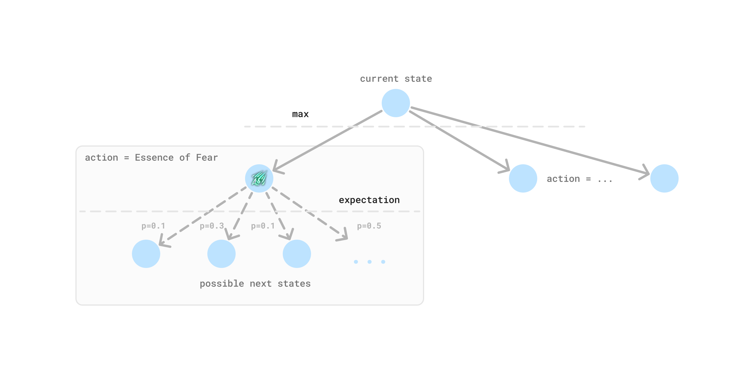
A popular algorithm for finding optimal actions in games is Minimax search. In our case, we have one player instead of two, and our environment is stochastic. We can still use this approach by replacing the min operation with an expectation, also called expectimax. This approach has been applied to games such as 2048 to find optimal plays. Can we build a game tree to find the optimal crafting strategy? It would look something like this:
It turns out, the answer is no. At least not easily without a lot of additional heuristics and tricks. Our problem has two properties that makes this approach difficult to apply:
- Cyclic Graph - Many crafting actions result in identical states, as we’ve seen in the example above. And certain randomizing currencies can transport you into a large number of states. Not only do we not have a tree, but our graph is both dense and highly cyclic. If we had a DAG (Directed Acyclic Graph) we could reduce redundant computation by aliasing identical states using transposition tables. This is true for many board games. In some cases it’s possible to break cycles using heuristics, but in our case this would result in incorrect estimates since cycles are a result of the environment stochasticity that we must take an expectation over.
- Unprunable large branching factor - The space of possible items is huge. With ~100 different spawnable modifiers on an item base we have on the order of \(10^{12}\) possible outcomes for randomizing actions. The number of valid states is much less than this due to restrictions on which modifiers can appear together, but it is still extremely large. Dealing with large branching factors in tree searches can be done using techniques like alpha-beta pruning to avoid exploring unpromising branches. But in our case the branching factor is due to stochasticity in the environment, which we must take an expectation over, meaning that we cannot easily prune away paths like we could when choosing an action.
What about MCTS? #
Monte Carlo Tree Search (MCTS), popular for its role in AlphaGo, is an alternative that allows us to explore the game tree using sampling techniques and confidence bounds for exploration. Instead of rolling out the full tree, we would run Monte Carlo simulations to estimate the value of intermediate nodes. This solves the branching factor issue by building an “asymmetric” tree. And while MCTS can be applied to graphs instead of trees with some modifications, it still requires a DAG for its backpropagation algorithm to be sound if we want to share computation across states.
Formalizing the problem as a Markov Decision Process #
Fortunately, our problem fits neatly into the framework of Markov Decision Processes (MDPs) and Reinforcement Learning. An MDP is defined by a tuple \((S, A, P, R)\) where:
- \(S\) is the set of possible states. Each \(s \in S\) represents the current state of the item being crafted. We’ll get to how we represent the state using a feature vector later.
- \(A_s\) is the set of actions available in state \(s\). An action \(a \in A_s\) corresponds to modifying the item using a crafting currency.
- \(P(s_{t+1} | s_t, a)\) is the transition function. Given a state \(s_t\) and an action \(a\), it defines the probability distribution over the next state \(s_{t+1}\), i.e. the possible outcomes of a crafting step.
- \(R(s_t, a)\) is the reward function. It defines the reward received from taking action \(a\) in state \(s_t\). We’ll discuss it more below.
Solving an MDP means finding a policy \(\pi(s)\) that maps each state to an optimal action. Optimal in what sense? This policy typically maximizes the expected sum of rewards over time, i.e. the average total reward over possible trajectories. One way to find such a policy is by learning a state-action value function, also called q-function, \(Q(s, a)\). This function assigns a value to each state-action pair, representing the expected sum of rewards when taking action \(a\) in state \(s\) and following the optimal policy thereafter. When you have the optimal q function, the optimal policy is easily derived by picking the best action in each state: \(\pi(s) = \text{argmax}_a Q(s, a)\).
Depending on what we want to optimize, we can define the reward function in different ways. One useful reward function for our crafting problem is a constant \(R(s_t, a) = -1\) for all states and actions. This would encourage the agent to craft the item in as few steps as possible. The total reward for 50 steps (-50) is larger than the total reward for 100 steps (-100), making it preferable. In this case, the Q function would represent the expected number of steps needed to reach the target item given the current state and next action.
Another option is to define the reward as the cost of the action being taken, \(R(s_t, a) = -\text{cost}(a)\). This would encourage the agent to craft the item in the cheapest way possible. We can obtain an estimate of the cost for various actions from the economy data available on poeninja. In this case, the Q function represents the expected cost of crafting the target item from a given state. Low cost may come at the expense of a long crafting process. In PoE, this is not uncommon. Because certain transition probabilities are very low, it may take thousands of steps to craft an item in the most economical way. Some players prefer to spend more, but be done quickly.
The transition function \(P(s_{t+1} | s_t, a)\) is is what makes our problem difficult. Knowing \(P\) means you know the dynamics of the environment. In combination with knowing the reward function (which we always do), this is also called a model of the environment and we can use it to simulate transitions without needing to touch the real world. In deterministic fully observable board games such as Chess or Go we know the rules of the game and have a perfect model. In other problem domains, such as robotics, we may not know the dynamics of the environment, or we may be unable to express them in closed form. The environment could also be stochastic, e.g. wind could push your robot into random directions.
In our case, we know the dynamics of the environment in theory from datamined information available on sites such as craftofexile.com and poedb.tw. However, for many actions we cannot express \(P(s_{t+1} | s_t, a)\) directly because the distribution of possible outcomes is too large. We also cannot easily factor this categorical distribution. However, we can quite easily sample transitions \(s_{t+1} \sim P(s_{t+1} | s_t, a)\) by writing code that simulates each currency action. That is, we have sample model but not a distribution model of our environment. For example, the implementation of an Orb of Annulment, which removes a random prefix or suffix from an item, looks something like this in my Rust implementation:
impl Currency for Annulment {
    fn apply(self, item: &mut Item) -> Result<()> {
        // Handle metamods
        let mmf = MetamodFilter::from_existing_mods(item.all_mods());

        // Check for non-fractured candidate mods to remove
        // Filter out mods that cannot be removed
        let existing_prefixes = item.mods.for_generation_type(ModGenerationType::Prefix);
        let existing_suffixes = item.mods.for_generation_type(ModGenerationType::Suffix);
        let candidate_mods = existing_prefixes
            .chain(existing_suffixes)
            .filter(|m| mmf.filter_existing(m))
            .filter(|m| mmf.filter_new(m))
            .collect::<Vec<_>>();

        if candidate_mods.is_empty() {
            return Err(CurrencyError::NoModsToRemove.into());
        }

        // Remove a random mod
        let mut rng = thread_rng();
        let mod_to_remove = candidate_mods.choose(&mut rng).unwrap();
        item.mods.mods_mut().remove(mod_to_remove);

        Ok(())
    }
}
(I am sorry for mixing Python pseudocode with Rust code in this post. My real implementation is in Rust and those snippets are copied directly from my codebase. But I prefer Python pseudocode for getting high-level ideas across)
Item representation #
We need to represent the state space \(S\) in a way that’s appropriate for learning a good policy. Naively, each item could be represented as a bitstring where each bit corresponds to the presence of a specific modifier. We often have 100+ spawnable modifiers for an item base. Let’s say we cap this at 512. A set of item modifiers could be represented as 512 bits 0001....0, with a total of \(2^{512}\) possible combinations. Because an item can have at most 3 prefixes and 3 suffixes, only a small portion of this space is valid and the representation is quite sparse.
One problem with such a representation is that it does not easily allow for generalization. Imagine the Q-function \(Q(s, a)\) as a table that assigns a value to each state-action pair. With the naive representation we would learn a different value for each possible combination of modifiers, even though many states are similar. For example, if we have an item with two modifiers we want and an additional modifier we don’t care about, it typically (there are exceptions) does not matter what exactly this additional modifier is. It would be better if our representation could capture this. In other words, we want a more compact feature vector suitable for Machine Learning.
We have a few choices here. We can either design a feature vector by hand, or we can use a Neural Network (or similar) to learn a good feature representation. While I believe the Neural Network approach would work and has the benefit of being more generic, interleaving Neural Network training and Reinforcement Learning opens a whole new can of worms. It would probably increase our iteration time by 10-100x. So let’s see if we can get away with hand-crafted features first and come back to the idea of learning features later.
The intuition behind our feature representation is that it should capture the difference between our target item and the current state of the item. Let’s say our target item has 5 modifiers \(m_1, \dots, m_5\) and our current state contains 3 of these modifiers \(m_1, m_3, m_5\). We can represent the state as a bitstring of length 5, where each a bit is 1 if the modifier is present and 0 otherwise: 10101. More formally, if \(T = \{m_1, \dots, m_n\}\) is the set of modifiers on the target item and \(X \subseteq T\) is the set of modifiers on the current item our feature vector can be written as \(b_n \dots b_1\) where:
$$ \begin{aligned} b_i = \begin{cases} 1 & \text{if } m_i \in X, \\ 0 & \text{if } m_i \notin X \end{cases} \end{aligned} $$
(An nice side effect of a bitstring representation is that we can efficiently compare two states using bitwise operations)
Knowing which target modifiers are present should allow our agent to make an informed decision about what to do next. But this representation is missing a crucial bit of information: How full is our item? If we have 3 ouf of 5 matching modifiers but our item is at the maximum of 6 modifiers, 3 of which are irrelevant to us, we can’t add new modifiers. In such a case we may need to use an Orb of Annulment and hope that we remove one of the irrelevant modifiers to continue crafting. This is quite a different state from hitting 3 out of 5 modifiers and still having 3 open spaces on the item. Thus, we also add the total number of prefixes and suffixes on the item to our feature vector. Let’s look at an example:
Target modifier IDs:    3 (prefix), 9 (prefix), 5 (suffix), 1 (suffix), 8 (suffix)
Current modifier IDs:   3 (prefix), 5 (suffix), 1 (suffix), 4 (suffix)
Feature vector: 01101|1|3
In this example, we are missing the modifier at index 2 (id = 9) and index 5 (id = 8), and we have one irrelevant modifier with id = 4. The item has 1 prefix, and 3 suffixes.
This is a pretty compact feature representation, but it has some important limitations:
- Mod families - In PoE, each modifier may belong to one or more mod families. Only one modifier from any given family may appear on an item. This restriction changes the distribution of possible outcomes of each action. Our feature representation does not capture which irrelevant mods are on the item, and hence does not capture which mod families they belong to. Note that we are still capturing the mod families of target mods because we specify those explicitly. We are only missing those of non-target mods. In many crafts this is not a big problem, but in some cases this information can be important.
- Mod tags - Similiar to mod families, mods can have associated tags. Certain metamods interact with these tags and change the distribution of possible outcomes depending on the tags present. Again, we are capturing the tags of target mods. But we are missing those of non-target mods.
- Fractures - Modifiers on items can be fractured, meaning that they are fixed on the item and cannot be modified or removed through actions. Because our feature representation does not capture which mods are fractured, we are not allowed to change the fractures as part of the crafting process. While it would be nice to have fracturing as part of the optimization, this is not a big problem in practice beccause fractures are typically fixed at the start of the crafting process. We can simply treat each possible fracture as a different crafting problem.
Despite these limitations, the above representation will be sufficient to solve a good portion of crafting problems in PoE.
(Update: I extended the feature representation with both mod families and mod tags after writing this post. While this significantly increased the computation required to solve the MDP, the approach presented here continued to work just fine)Side note: Sim-to-Real Gap and modifier tags #
In Reinforcement Learning, The Sim-to-Real gap (Simulation to Reality gap) is a term used to descripe the discrepancy between how an agent trained in a simulation behaves in the real world. There are many factors that can lead to discrepeancies. A simplified model of the world using a featurized representation of the state that does not capture all aspects of the real world is one of them. In my early experiments, I ran into this exact issue because our featurized representation did not include mod tags. The metamod “Cannot roll Attack Modifiers” changes which mods may be removed by an Orb of Annulment. Training an agent on a model using the featurized representation, it learned to use an Annuls in a certain state. However, if this state included a mod with the “Attack” tag, the agent would deterministically remove an unwanted modifier. In the real world, this could result in an infinite loop of the agent deterministically removing a target modifier and crafting it again. In this case, the problem was easily avoided by adding a simple heuristic (see below) as opposed to expanding the feature representation.
Learning a Model #
In featurized state space we can represent the distribution of outcomes for each action as a table in memory. We can also represent \(Q(s, a)\), where each entry is the expected return of taking action \(a\) in state \(s\), as a table and don’t need a function approximator such as a Neural Network. How do we learn such a table? We could use model-free control algorithms such as Q-Learning which do not require the full distribution \(P(s_{t+1} | s_t, a)\), only the ability to sample transitions and simulate the crafting process.
That would work, but we’ll take a slightly different approach here. Instead of learning \(Q(s, a)\) directly, we learn \(P(s_{t+1} | s_t, a)\) where \(s\) is now our feature vector instead of the original item representation. In other words, we learn a model of the dynamics of the crafting process in feature space. With such a model we can use it to solve the MDP using q-value iteration (dynamic programming). Because our space of \(|S| |A|\) is rather small, we can learn a model by iterating over all possible states and actions, sampling each transition N times, and counting the outcomes. We only need enough samples to get a good enough estimate of the outcome distribution. In my experiments, I found that \(10^5\) samples per action were sufficient. With a larger feature representation, we would need more samples.
Why learn a model of the environment and solve the MDP instead of directly learning a policy with model-free RL algorithms? There are some benefits to having a model. For example, you can freely change the reward function without needing to re-learn the model. But the short answer is that it seems to work better for our problem domain. In my experiments, Q-Learning and its variations took 10+ minutes to converge to a good policy. They were also quite sensitive to hyperparameters such as the learning rate, exploration rate and algorithm, and decay factors. In contrast, the model-based approach converged in seconds and required no hyperparameter tuning. The tradeoff is that this approach may not work for much larger state spaces. We are naively exploring the full space of possible outcomes for each action, and we can only get away with this because our featurized space is small.
In pseudoce, a naive implementation of learning a model is as simple as this:
# Count all transitions
for s in all_states:
    for a in valid_actions(state):
        for _ in range(NUM_SAMPLES):
            s_next = apply_action(s, a)
            model[(s, a)][s_next] += 1
            counts[(s, a)] += 1

# Normalize the probabilities
for (s, a) in model:
    model[(s, a)] /= counts[(s, a)]
In practice, it’s a little bit more tricky. Before looking at more realistic code, let’s talk about a few optimizations we can make.
Afterstates #
Let’s think about what happens when we apply an Essence to an item. An Essence adds a fixed modifier (depending on the Essence type) and randomizes the rest of the item. In this case, the outcome distribution is independent of the current item state. We only need to learn the transition probabilities for \((s, a)\) pairs where \(a\) is some Essence once, and can re-use the result for all \(s\). Such cases are also called afterstates. They are common in board games like Tic-Tac-Toe where the value of an action is determined by the state of the board after the action is taken. It doesn’t what the board state was before, and you can get to the same board state in multiple ways. In our code, we can replace the \((s,a)\) tuple in \(P(s,a)\) with an enum:
pub enum StateActionAlias<S> {
    Pair((S, Action)),
    AfterEssence(Action),
    // more possible afterstates ...
}
In practice, we need to be a bit careful with this. Requirements often change. For example, applying an Essence only leads to the same distribution if we don’t change fractured modifiers as part of the crafting process. Currently we don’t, but in the future we might, and then our afterstates will lead to incorrect results.
Pruning the action space with heuristics #
We can use heuristics to filter out obviously bad actions based on the current state, reducing the size of the action space. For example, using the crafting bench to deterministically add a modifier to an item is almost always the last step in a craft. It’s only a good idea when the rest of the item is already done.
Use full distributions when possible #
We’ve already discussed that we cannot express the full distribution of outcomes in general. But for some actions we can. In such cases we don’t need to waste computation trying to approximate the distribution using sampling techniques. We can just update the model with the distribution directly. Only for state-action pairs where the distribution is too large do we need to sample transitions. I did not implement this optimization in my code because performance was good enough for my use case already, but it’s something that will come in handy when scaling up to larger state spaces.
Implementation #
With these optimizations, the implementation of learning a model looks roughly as follows. Unlike the pseudocode above, we are no longer iterating over all states and actions. Instead, we “naturally” explore the state space in depth-first manner by sampling the transitions and adding unseen states to a queue. The output of the model learning process is a table representing \(P(s_{t+1} | s_t, a)\).
/// Learn a table model by sampling transition probabilities
pub fn learn_model_v2<S, F>(
    // description of the crafting task
    task: rl::CraftingTask,
    // number of samples per state-action pair
    samples_per_state: usize,
    // alias function mapping a state-action pair to an alias
    alias_fn: F,
    // state featurizer function
    state_featurizer: impl Fn(&Item) -> S,
) -> Result<TableModelV2<S, F>>
where
    S: rl::StateRepr,
    F: Fn(&S, Action) -> StateActionAlias<S>,
{
    let mut model = TableModelV2Builder::new(alias_fn);

    // Keeps track of states we have already learned
    let mut done_states = HashSet::new();

    // Keeps track of the states we need to learn, starting with the initial item state
    let mut queue = Vec::new();
    queue.push(task.base.clone());

    loop {
        let item = match queue.pop() {
            Some(item) => item,
            // We are done
            None => break,
        };

        // If the state is terminal we don't need to sample further transitions from it
        if task.target.is_item_done(&item) {
            continue;
        }

        // Compute the feature representation of the ite,
        let features = state_featurizer(&item);

        // Mark the state as done
        done_states.insert(features);

        // Get the valid actions for the item
        let actions = task.action_space.all_for_item(&item);

        // For each action, sample the transition N times
        for action in actions {

            // If we have already learned a model for this state-action pair, skip it
            if model.check_alias(features, action) {
                continue;
            }

            // Sample the transition N times
            for _ in 0..samples_per_state {
                let mut item = item.clone();
                action.apply(&mut item)?;

                let next_features = state_featurizer(&item);

                // Update the model with the transition
                model.update(features, action, next_features);

                // If we have not learned a model for the resulting state yet, add it to the queue
                if !done_states.contains(&next_features) {
                    done_states.insert(next_features); // avoid duplicates
                    queue.push(item.clone());
                }
            }
        }
    }

    // Normalizes transition probabilities
    Ok(model.build())
}
Solving the MDP #
With a learned distribution model of the environment (in featurized space) it is now trivial to solve the resulting MDP using q-value iteration, which is the continuous application of the Bellman Equation that expresses the optimal value of a state-action pair in terms of the expected reward of taking the action and the value of the next state:
$$ \begin{aligned} Q(s, a) &= R(s, a) + \gamma \sum_{s’} P(s’ | s, a) \max_{a’} Q(s’, a’) \ \end{aligned} $$
Here, \(\gamma\) is the discount factor, which is mostly important for convergence properties in non-episodic tasks. We always set it to 1 because we don’t need or want to discount future rewards. The algorithm converges once the change in the value function falls below a threshold \(\theta\). In our code, we also return the state-value function \(V(s) = \max_a Q(s, a)\), which is the expected return when following optimal policy from that state. We do this only because it’s “free” to compute during the algorithm and we might as well have it for debugging purposes, but we don’t use it for anything important.
/// Compute the optimal state-action value function using the Bellman equation
pub fn value_iteration(&self, gamma: f64, theta: f64) -> (ValueFn<S>, StateActionValueFn<S>) {
    // State-value function
    let mut v = HashMap::new();
    // State-action value function
    let mut q = HashMap::new();

    let mut i = 0;
    loop {
        let mut delta: f64 = 0.0;

        // For each state, update the value function
        for state in self.model.state_space() {
            let mut max_q = f64::NEG_INFINITY;
            let state = *state;

            // For each action in the state
            for action in self.model.valid_actions(&state).unwrap().iter() {

                // Compute the expected value of the action by taking the expectation over the next states
                let action = *action;
                let transitions = self.model.distribution(state, action);
                let reward = (self.reward_fn)(&state, action);
                let mut new_q_value = reward;
                for (next_state, prob) in transitions {
                    let next_value = v.get(&next_state).unwrap_or(&0.0);
                    new_q_value += gamma * prob * next_value;
                }

                // Update and track the maximum delta
                let q_value = q.entry((state, action)).or_insert(0.0);
                delta = delta.max((new_q_value - *q_value).abs());
                *q_value = new_q_value;

                max_q = max_q.max(new_q_value);
            }

            // Update the state-value function with the maximum action value
            v.insert(state, max_q);
        }

        // check for convergence
        if delta < theta {
            break;
        }
        i += 1;
    }

    tracing::info!(%i, %theta, "q-value iteration done");
    (v, q)
}
From the Q-function we can now derive our policy \(\pi(s) = \text{argmax}_a Q(s, a)\) which maps each state to the optimal action to take.
Example Crafts #
A good test case for our algorithm is this leaguestart Boneshatter Axe. The crafting process is rather simple, but in the second step the optimal action is to use a “Cannot Roll Attack Mods” metamod in combination with an Orb of Annulment, which wouldn’t be immediately obvious to many players. Let’s see if our algorithm discovers this optimal policy.
Optimizing for Path Length #
Remember that setting the reward function to a constant -1 encourages the agent to craft the item in as few steps as possible. In this case, the values of \(Q(s, a)\) represent the expected remaining number of steps to reach the target item from a given state. Let’s look at some of these q-values. The full table would be too large to show, but here is a slice, mapping our featurized representation and action to the expected number of remaining steps:
[Magic |00000100|1|0] -> Regal      | -131.12
[Magic |00000100|1|1] -> Regal      | -131.12
[Magic |00000101|1|1] -> Regal      | -132.11
[Magic |00000110|1|1] -> Regal      | -131.13
[Rare  |00000100|1|0] -> Contempt(7) | -130.13
[Rare  |00000100|1|1] -> Contempt(7) | -130.12
[Rare  |00000100|1|2] -> Contempt(7) | -130.13
[Rare  |00000100|1|3] -> Contempt(7) | -130.13
[Rare  |00000100|2|0] -> Contempt(7) | -130.12
[Rare  |00000100|2|1] -> Contempt(7) | -130.13
[Rare  |00000100|2|2] -> Contempt(7) | -130.13
[Rare  |00000100|2|3] -> Contempt(7) | -130.13
[Rare  |00000110|1|3] -> Contempt(7) | -130.13
[Rare  |00000110|2|1] -> Contempt(7) | -130.12
[Rare  |00001110|3|3] -> Contempt(7) | -130.13
[Rare  |00001111|2|2] -> RemoveBench | -131.12
[Rare  |00010110|2|1] -> Contempt(7) | -130.12
[Rare  |00010110|2|2] -> Contempt(7) | -130.12
[Rare  |00010110|2|3] -> Contempt(7) | -130.13
[Rare  |00010111|2|2] -> RemoveBench | -131.12
[Rare  |00010111|2|3] -> RemoveBench | -131.12
[Rare  |00011100|3|0] -> BenchCraft(StrIntMasterItemGenerationCanHaveMultipleCraftedMods) | -3.00
[Rare  |00011100|3|1] -> BenchCraft(IntMasterItemGenerationCannotRollAttackAffixes) | -8.01
[Rare  |00011100|3|2] -> BenchCraft(IntMasterItemGenerationCannotRollAttackAffixes) | -11.03
[Rare  |00011100|3|3] -> Annulment  | -59.56
[Rare  |00011101|3|1] -> RemoveBench | -4.00
[Rare  |00011101|3|2] -> Annulment  | -7.01
[Rare  |00011101|3|3] -> Annulment  | -10.03
[Rare  |00011110|3|1] -> BenchCraft(EinharMasterLocalIncreasedAttackSpeed3) | -2.00
[Rare  |00011110|3|2] -> BenchCraft(IntMasterItemGenerationCannotRollAttackAffixes) | -8.51
[Rare  |00011110|3|3] -> RemoveBench | -12.03
[Rare  |00011111|3|2] -> RemoveBench | -4.00
[Rare  |00011111|3|3] -> Annulment  | -7.51
[Rare  |00100100|1|1] -> Contempt(7) | -130.13
[Rare  |00111110|3|2] -> BenchCraft(EinharMasterLocalIncreasedAttackSpeed3) | -1.00
[Rare  |00111110|3|3] -> RemoveBench | -9.01
[Rare  |00111111|3|3] -> Annulment  | -4.00
[Rare  |01000100|1|1] -> Contempt(7) | -130.12
[Rare  |01000100|1|2] -> Contempt(7) | -130.13
[Rare  |01000100|1|3] -> Contempt(7) | -130.13
[Rare  |01000101|1|2] -> RemoveBench | -131.12
[Rare  |01010100|2|1] -> Contempt(7) | -130.12
[Rare  |01010111|2|3] -> RemoveBench | -131.12
[Rare  |01011110|3|2] -> BenchCraft(JunMaster2DoubleDamageChance2h2) | -1.00
[Rare  |01011110|3|3] -> RemoveBench | -9.01
[Rare  |01011111|3|3] -> Annulment  | -3.51
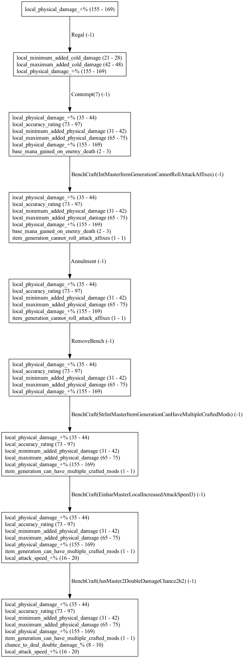
The perhaps most interesting entry is the value of the optimal action in the initial state, which is [Magic |00000100|1|0] in our case. This tells us the that expected total reward, i.e. the expected number of steps to craft the item from scratch, is -131.12. Most of these steps consist of spamming Essences of Contempt until we are lucky to hit the modifiers we want. Once we hit these modifiers, we can finish up the item with a few deterministic benchcrafts. The following picture shows an example rollout of our learned optimal policy with pruning of repeated steps for visualization. Since the expected number of steps is 131, the full graph for an average craft would be too large to show here. Each node shows the current item mods and each edge shows the action taken and reward received. Our learned optimal policy matches the expert policy from the guide above, including the use of the metamod in the second stage.
We can also visualize the the learned model for \(P(s_{t+1} | s_t, a)\) as a graph. Nodes represent states and edges represent transitions. I colored the nodes according to the number of matching target mods and pruned the action space to trim down the graph a bit for visualization.
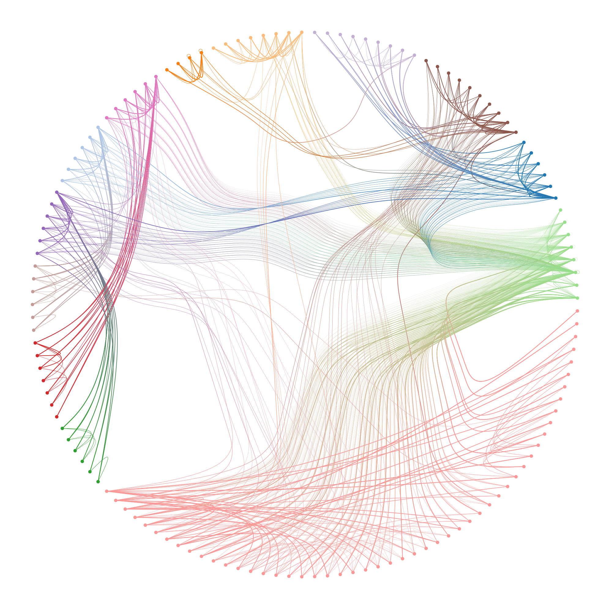
For comparison, here is an untrimmed model graph with subsampled edges for a slightly more complex crafting problem with a larger reachable state space:

Optimizing for Cost #
Instead of using a step penalty, let’s try using the cost of each action as the reward function. This will give us the expected cost of crafting the target item. In PoE, there is no standard currency such as gold. Instead, players trade various currencies against others. The most common currency used as a numeraire for trading is the Chaos Orb. We can use data from poe.ninja to estimate the price of each currency item denominated of Chaos Orbs. For example, the Essence of Contempt used in the craft above has the following price history and currently sits at 1.6 Chaos Orbs. With this data, we can implement a reward function that matches each action to its cost.
Before changing the optimization and solving the MDP with a different reward function, let’s run our optimal policy from above with the cost reward function. In other words, let’s see what the expected cost of the item when is when we optimize for path length. The following is the average cost from 10,000 simulation runs.
Amount | Currency
------ | --------
  8.00 | Chaos Orb
125.71 | Deafening Essence of Contempt
  4.10 | Divine Orb
  1.00 | Exalted Orb
  2.64 | Orb of Annulment
  1.00 | Orb of Scouring
  1.00 | Regal Orb
------ | --------
665.05 | Chaos Equivalent
As expected, we are using a lot of Essences of Contempt. In our craft example above, the optimal policy would be identical whether we optimize for cost or path length. This is often the case. After all, a shorter path means using less currency. But there are exceptions. Let’s look at one. Let’s say our goal is to craft the following Magic Jewel with two modifiers:
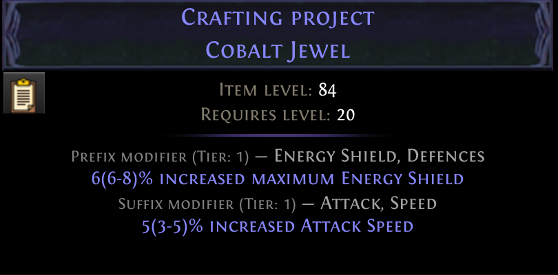
A magic item can have at most 2 modifiers and most currencies can only be applied to rare items. Thus, the state and action space for this problem is rather small and we can look at the full table. When optimizing for the shortest path, we get the following policy.
[Magic |00000000|0|1] -> Alteration | -654.16
[Magic |00000000|1|0] -> Alteration | -654.16
[Magic |00000000|1|1] -> Alteration | -654.17
[Magic |00000001|1|0] -> Augment    | -623.21
[Magic |00000001|1|1] -> Annulment  | -639.62
[Magic |00000010|0|1] -> Augment    | -624.04
[Magic |00000010|1|1] -> Annulment  | -640.02
We need on average ~650 steps to finish the craft. By running simulations with the cost as the reward function we estimate the following currency usage. Note that we are still optimizing for path length here, we only change the reward function for our evaluation runs, but not our training runs.
Amount | Currency
------ | --------
569.54 | Orb of Alteration
 43.88 | Orb of Annulment
 29.65 | Orb of Augmentation
------ | --------
281.44 | Chaos Equivalent
Most of our steps are spamming Orbs of Alteration. If we happen to hit one of the two desired mods, we can try our luck with an Orb of Annulment followed up by an Orb of Augmentation. That’s the shortest way to get the result we want. However, Orbs of Annulment are more expensive than Orbs of Alteration. So what happens if we optimize for cost instead? Now, the policy changes to:
[Magic |00000000|0|1] -> Alteration | -187.19
[Magic |00000000|1|0] -> Alteration | -187.18
[Magic |00000000|1|1] -> Alteration | -187.18
[Magic |00000001|1|0] -> Augment    | -182.23
[Magic |00000001|1|1] -> Alteration | -187.18
[Magic |00000010|0|1] -> Augment    | -182.08
[Magic |00000010|1|1] -> Alteration | -187.18
 Amount | Currency
 ------ | --------
1351.14 | Orb of Alteration
  19.33 | Orb of Augmentation
 ------ | --------
 204.02 | Chaos Equivalent
The q-values in the tables are not directly comparable since the former is the number of remaining steps and the latter is the remaining cost in terms of Chaos Orbs. But we can see that the optimal policy and total expected cost have changed. Instead of spending 281.44 Chaos Orbs on average we are now spending 204.02 and we are no longer using the more expensive Orb of Annulment. However, we need ~1350 steps to get the result we want. That’s a lot of clicks.
Closing Thoughts #
We’ve only scratched the surface of what we can do with an RL-based approach to crafting in PoE. Here are a few ideas for further exploration.
More expressive state representation #
Our compact state representation limits what types of crafting actions we can support. For example, we cannot support changing fractures with a Fracturing Orb or Veiled Modifiers. With a few more optimizations I believe that we can increase the size of our current state space by a factor of 10-100 without running into performance issues. Beyond that we would likely need a smarter approach to train our model that does not rely on the naive exploration of the state space. Or we would need a function approximator such as a Neural Network to help us generalize.
Model-free RL #
In my experiments, model-free RL algorithms such as q-learning were more noisy and took significantly longer to converge to a good policy than our model-based approach. However, they can avoid unpromising parts of the state space with a good exploration algorithm. On one hand, that’s great because it helps us avoid exploring the full space. On the other hand, that’s another algorithm to tune and optimize with hyperparameters. But with a few tricks to speed up convergence I could see model-free approaches being more sample-efficient than our current approach. We could also combine both approaches and iterate between model and policy improvement.
Combining Item Crafting with Trade APIs #
The expected cost of crafting an item could be seen as its “fair market price”. Using PoE’s trade website and API we could find items that are selling well above their expected crafting cost and use this information to find the most profitable crafts automatically.
Function approximation, Neural Networks, Policy Gradients #
We could use a combination of one-hot encodings for our item representation and let a Neural Network learn the necessary feature vectors. With a differentiable function approximator we could also try learning a policy using a policy-gradient approach instead of going through Q-values.