Deep Learning for Chatbots, Part 2 – Implementing a Retrieval-Based Model in Tensorflow

The Code and data for this tutorial is on Github.

Retrieval-Based bots #

In this post we’ll implement a retrieval-based bot. Retrieval-based models have a repository of pre-defined responses they can use, which is unlike generative models that can generate responses they’ve never seen before. A bit more formally, the input to a retrieval-based model is a context \(c\) (the conversation up to this point) and a potential response \(r\). The model outputs is a score for the response. To find a good response you would calculate the score for multiple responses and choose the one with the highest score.

But why would you want to build a retrieval-based model if you can build a generative model? Generative models seem more flexible because they don’t need this repository of predefined responses, right?

The problem is that generative models don’t work well in practice. At least not yet. Because they have so much freedom in how they can respond, generative models tend to make grammatical mistakes and produce irrelevant, generic or inconsistent responses. They also need huge amounts of training data and are hard to optimize. The vast majority of production systems today are retrieval-based, or a combination of retrieval-based and generative. Google’s Smart Reply is a good example. Generative models are an active area of research, but we’re not quite there yet. If you want to build a conversational agent today your best bet is most likely a retrieval-based model.

The Ubuntu Dialog Corpus #

In this post we’ll work with the Ubuntu Dialog Corpus (paper, github). The Ubuntu Dialog Corpus (UDC) is one of the largest public dialog datasets available. It’s based on chat logs from the Ubuntu channels on a public IRC network. The paper goes into detail on how exactly the corpus was created, so I won’t repeat that here. However, it’s important to understand what kind of data we’re working with, so let’s do some exploration first.

The training data consists of 1,000,000 examples, 50% positive (label 1) and 50% negative (label 0). Each example consists of a context, the conversation up to this point, and an utterance, a response to the context. A positive label means that an utterance was an actual response to a context, and a negative label means that the utterance wasn’t – it was picked randomly from somewhere in the corpus. Here is some sample data.

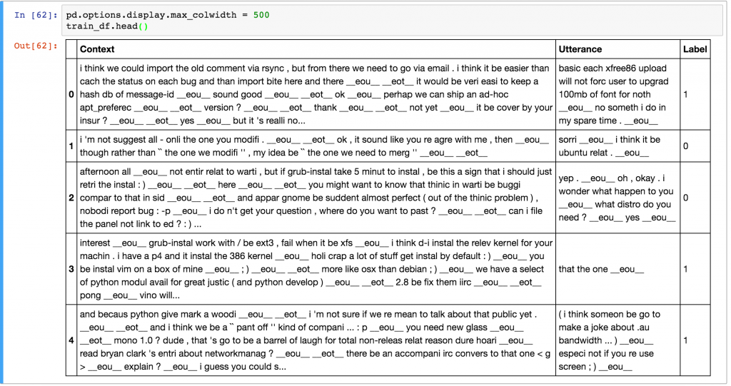
Note that the dataset generation script has already done a bunch of preprocessing for us – it has tokenized, stemmed, and lemmatized the output using the NLTK tool. The script also replaced entities like names, locations, organizations, URLs, and system paths with special tokens. This preprocessing isn’t strictly necessary, but it’s likely to improve performance by a few percent. The average context is 86 words long and the average utterance is 17 words long. Check out the Jupyter notebook to see the data analysis.

The data set comes with test and validations sets. The format of these is different from that of the training data. Each record in the test/validation set consists of a context, a ground truth utterance (the real response) and 9 incorrect utterances called distractors. The goal of the model is to assign the highest score to the true utterance, and lower scores to wrong utterances.

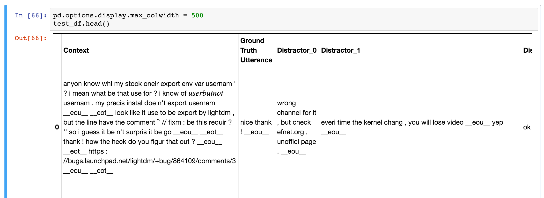
The are various ways to evaluate how well our model does. A commonly used metric is recall@k. recall@k means that we let the model pick the k best responses out of the 10 possible responses (1 true and 9 distractors). If the correct one is among the picked ones we mark that test example as correct. So, a larger k means that the task becomes easier. If we set k=10 we get a recall of 100% because we only have 10 responses to pick from. If we set k=1 the model has only one chance to pick the right response.

At this point you may be wondering how the 9 distractors were chosen. In this data set the 9 distractors were picked at random. However, in the real world you may have millions of possible responses and you don’t know which one is correct. You can’t possibly evaluate a million potential responses to pick the one with the highest score – that’d be too expensive. Google’s Smart Reply uses clustering techniques to come up with a set of possible responses to choose from first. Or, if you only have a few hundred potential responses in total you could just evaluate all of them.

Baselines #

Before starting with fancy Neural Network models let’s build some simple baseline models to help us understand what kind of performance we can expect. We’ll use the following function to evaluate our recall@k metric:

def evaluate_recall(y, y_test, k=1):
    num_examples = float(len(y))
    num_correct = 0
    for predictions, label in zip(y, y_test):
        if label in predictions[:k]:
            num_correct += 1
    return num_correct/num_examples

Here, y is a list of our predictions sorted by score in descending order, and y_test is the actual label. For example, a y of [0,3,1,2,5,6,4,7,8,9] Would mean that the utterance number 0 got the highest score, and utterance 9 got the lowest score. Remember that we have 10 utterances for each test example, and the first one (index 0) is always the correct one because the utterance column comes before the distractor columns in our data.

Intuitively, a completely random predictor should get a score of 10% for recall@1, a score of 20% for recall@2, and so on. Let’s see if that’s the case.

# Random Predictor
def predict_random(context, utterances):
    return np.random.choice(len(utterances), 10, replace=False)

# Evaluate Random predictor
y_random = [predict_random(test_df.Context[x], test_df.iloc[x,1:].values) for x in range(len(test_df))]
y_test = np.zeros(len(y_random))
for n in [1, 2, 5, 10]:
    print("Recall @ ({}, 10): {:g}".format(n, evaluate_recall(y_random, y_test, n)))

Recall @ (1, 10): 0.0937632  
Recall @ (2, 10): 0.194503  
Recall @ (5, 10): 0.49297  
Recall @ (10, 10): 1  

Great, seems to work. Of course we don’t just want a random predictor. Another baseline that was discussed in the original paper is a tf-idf predictor. tf-idf stands for “term frequency – inverse document frequency" and measures how important a word in a document is relative to the whole corpus. Without going into too much detail (you can find many tutorials about tf-idf on the web), documents that have similar content will have similar tf-idf vectors. Intuitively, if a context and a response have similar words they are more likely to be a correct pair. Many libraries such as scikit-learn come with built-in tf-idf functions, so it’s quite easy to use. Let’s build a tf-idf predictor and see how well it performs.

class TFIDFPredictor:
    def __init__(self):
        self.vectorizer = TfidfVectorizer()

    def train(self, data):
        self.vectorizer.fit(np.append(data.Context.values,data.Utterance.values))

    def predict(self, context, utterances):
        # Convert context and utterances into tfidf vector
        vector_context = self.vectorizer.transform([context])
        vector_doc = self.vectorizer.transform(utterances)
        # The dot product measures the similarity of the resulting vectors
        result = np.dot(vector_doc, vector_context.T).todense()
        result = np.asarray(result).flatten()
        # Sort by top results and return the indices in descending order
        return np.argsort(result, axis=0)[::-1]

# Evaluate TFIDF predictor
pred = TFIDFPredictor()
pred.train(train_df)
y = [pred.predict(test_df.Context[x], test_df.iloc[x,1:].values) for x in range(len(test_df))]
for n in [1, 2, 5, 10]:
    print("Recall @ ({}, 10): {:g}".format(n, evaluate_recall(y, y_test, n)))

Recall @ (1, 10): 0.495032  
Recall @ (2, 10): 0.596882  
Recall @ (5, 10): 0.766121  
Recall @ (10, 10): 1  

We can see that the tf-idf model performs significantly better than the random model. It’s far from perfect though. The assumptions we made aren’t that great. First of all, a response doesn’t necessarily need to be similar to the context to be correct. Secondly, tf-idf ignores word order, which can be an important signal. With a Neural Network model we can do a bit better.

Dual Encoder LSTM #

The Deep Learning model we will build in this post is called a Dual Encoder LSTM network. This type of network is just one of many we could apply to this problem and it’s not necessarily the best one. You can come up with all kinds of Deep Learning architectures that haven’t been tried yet – it’s an active research area. For example, the seq2seq model often used in Machine Translation would probably do well on this task. The reason we are going for the Dual Encoder is because it has been reported to give decent performance on this data set. This means we know what to expect and can be sure that our implementation is correct. Applying other models to this problem would be an interesting project.

The Dual Encoder LSTM we’ll build looks like this (paper):

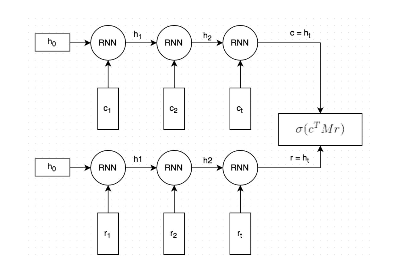
It roughly works as follows:

1. Both the context and the response text are split by words, and each word is embedded into a vector. The word embeddings are initialized with Stanford’s GloVe vectors and are fine-tuned during training (Side note: This is optional and not shown in the picture. I found that initializing the word embeddings with GloVe did not make a big difference in terms of model performance).

2. Both the embedded context and response are fed into the same Recurrent Neural Network word-by-word. The RNN generates a vector representation that, loosely speaking, captures the “meaning” of the context and response (c and r in the picture). We can choose how large these vectors should be, but let’s say we pick 256 dimensions.

3. We multiply c with a matrix M to “predict” a response r'. If c is a 256-dimensional vector, then M is a 256×256 dimensional matrix, and the result is another 256-dimensional vector, which we can interpret as a generated response. The matrix M is learned during training.

4. We measure the similarity of the predicted response r' and the actual response r by taking the dot product of these two vectors. A large dot product means the vectors are similar and that the response should receive a high score. We then apply a sigmoid function to convert that score into a probability. Note that steps 3 and 4 are combined in the figure.

To train the network, we also need a loss (cost) function. We’ll use the binary cross-entropy loss common for classification problems. Let’s call our true label for a context-response pair y. This can be either 1 (actual response) or 0 (incorrect response). Let’s call our predicted probability from 4. above y'. Then, the cross entropy loss is calculated as

$$ L= −y\log(y’) − (1 − y)\log(1−y’) $$

The intuition behind this formula is simple. If y=1 we are left with L = -ln(y'), which penalizes a prediction far away from 1, and if y=0 we are left with L= −ln(1−y'), which penalizes a prediction far away from 0.

For our implementation we’ll use a combination of numpy, pandas, Tensorflow and TF Learn (a combination of high-level convenience functions for Tensorflow).

Data Preprocessing #

The dataset originally comes in CSV format. We could work directly with CSVs, but it’s better to convert our data into Tensorflow’s proprietary Example format. (Quick side note: There’s also tf.SequenceExample but it doesn’t seem to be supported by tf.learn yet). The main benefit of this format is that it allows us to load tensors directly from the input files and let Tensorflow handle all the shuffling, batching and queuing of inputs. As part of the preprocessing we also create a vocabulary. This means we map each word to an integer number, e.g. “cat” may become 2631. The TFRecord files we will generate store these integer numbers instead of the word strings. We will also save the vocabulary so that we can map back from integers to words later on.

Each Example contains the following fields:

• context: A sequence of word ids representing the context text, e.g. [231, 2190, 737, 0, 912]
• context_len: The length of the context, e.g. 5 for the above example
• utterance A sequence of word ids representing the utterance (response)
• utterance_len: The length of the utterance
• label: Only in the training data. 0 or 1.
• distractor_[N]: Only in the test/validation data. N ranges from 0 to 8. A sequence of word ids representing the distractor utterance.
• distractor_[N]_len: Only in the test/validation data. N ranges from 0 to 8. The length of the utterance.

The preprocessing is done by the prepare_data.py Python script, which generates 3 files: train.tfrecords, validation.tfrecords and test.tfrecords. You can run the script yourself or download the data files here.

Creating an input function #

In order to use Tensorflow’s built-in support for training and evaluation we need to create an input function – a function that returns batches of our input data. In fact, because our training and test data have different formats, we need different input functions for them. The input function should return a batch of features and labels (if available). Something along the lines of:

def input_fn():
  # TODO Load and preprocess data here
  return batched_features, labels

Because we need different input functions during training and evaluation and because we hate code duplication we create a wrapper called create_input_fn that creates an input function for the appropriate mode. It also takes a few other parameters. Here’s the definition we’re using:

def create_input_fn(mode, input_files, batch_size, num_epochs=None):
  def input_fn():
    # TODO Load and preprocess data here
    return batched_features, labels
  return input_fn

The complete code can be found in udc_inputs.py. On a high level, the function does the following:

1. Create a feature definition that describes the fields in our Example file
2. Read records from the input_files with tf.TFRecordReader
3. Parse the records according to the feature definition
4. Extract the training labels
5. Batch multiple examples and training labels
6. Return the batched examples and training labels

Evaluation Metrics #

We already mentioned that we want to use the recall@k metric to evaluate our model. Luckily, Tensorflow already comes with many standard evaluation metrics that we can use, including recall@k. To use these metrics we need to create a dictionary that maps from a metric name to a function that takes the predictions and label as arguments:

def create_evaluation_metrics():
  eval_metrics = {}
  for k in [1, 2, 5, 10]:
    eval_metrics["recall_at_%d" % k] = functools.partial(
        tf.contrib.metrics.streaming_sparse_recall_at_k,
        k=k)
  return eval_metrics

Above, we use functools.partial to convert a function that takes 3 arguments to one that only takes 2 arguments. Don’t let the name streaming_sparse_recall_at_k confuse you. Streaming just means that the metric is accumulated over multiple batches, and sparse refers to the format of our labels.

This brings us to an important point: What exactly is the format of our predictions during evaluation? During training, we predict the probability of the example being correct. But during evaluation our goal is to score the utterance and 9 distractors and pick the best one – we don’t simply predict correct/incorrect. This means that during evaluation each example should result in a vector of 10 scores, e.g. [0.34, 0.11, 0.22, 0.45, 0.01, 0.02, 0.03, 0.08, 0.33, 0.11], where the scores correspond to the true response and the 9 distractors respectively. Each utterance is scored independently, so the probabilities don’t need to add up to 1. Because the true response is always element 0 in array, the label for each example is 0. The example above would be counted as classified incorrectly by recall@1 because the third distractor got a probability of 0.45 while the true response only got 0.34. It would be scored as correct by recall@2 however.

Boilerplate Training Code #

Before writing the actual neural network code I like to write the boilerplate code for training and evaluating the model. That’s because, as long as you adhere to the right interfaces, it’s easy to swap out what kind of network you are using. Let’s assume we have a model function model_fn that takes as inputs our batched features, labels and mode (train or evaluation) and returns the predictions. Then we can write general-purpose code to train our model as follows:

estimator = tf.contrib.learn.Estimator(
model_fn=model_fn,
model_dir=MODEL_DIR,
config=tf.contrib.learn.RunConfig())

input_fn_train = udc_inputs.create_input_fn(
mode=tf.contrib.learn.ModeKeys.TRAIN,
input_files=[TRAIN_FILE],
batch_size=hparams.batch_size)

input_fn_eval = udc_inputs.create_input_fn(
mode=tf.contrib.learn.ModeKeys.EVAL,
input_files=[VALIDATION_FILE],
batch_size=hparams.eval_batch_size,
num_epochs=1)

eval_metrics = udc_metrics.create_evaluation_metrics()

# We need to subclass theis manually for now. The next TF version will
# have support ValidationMonitors with metrics built-in.
# It's already on the master branch.
class EvaluationMonitor(tf.contrib.learn.monitors.EveryN):
def every_n_step_end(self, step, outputs):
  self._estimator.evaluate(
    input_fn=input_fn_eval,
    metrics=eval_metrics,
    steps=None)

eval_monitor = EvaluationMonitor(every_n_steps=FLAGS.eval_every)
estimator.fit(input_fn=input_fn_train, steps=None, monitors=[eval_monitor])

Here we create an estimator for our model_fn, two input functions for training and evaluation data, and our evaluation metrics dictionary. We also define a monitor that evaluates our model every FLAGS.eval_every steps during training. Finally, we train the model. The training runs indefinitely, but Tensorflow automatically saves checkpoint files in MODEL_DIR, so you can stop the training at any time. A more fancy technique would be to use early stopping, which means you automatically stop training when a validation set metric stops improving (i.e. you are starting to overfit). You can see the full code in udc_train.py.

Two things I want to mention briefly is the usage of FLAGS. This is a way to give command line parameters to the program (similar to Python’s argparse). hparams is a custom object we create in hparams.py that holds hyperparameters, nobs we can tweak, of our model. This hparams object is given to the model when we instantiate it.

Creating the model #

Now that we have set up the boilerplate code around inputs, parsing, evaluation and training it’s time to write code for our Dual LSTM neural network. Because we have different formats of training and evaluation data I’ve written a create_model_fn wrapper that takes care of bringing the data into the right format for us. It takes a model_impl argument, which is a function that actually makes predictions. In our case it’s the Dual Encoder LSTM we described above, but we could easily swap it out for some other neural network. Let’s see what that looks like:

def dual_encoder_model(
    hparams,
    mode,
    context,
    context_len,
    utterance,
    utterance_len,
    targets):

  # Initialize embedidngs randomly or with pre-trained vectors if available
  embeddings_W = get_embeddings(hparams)

  # Embed the context and the utterance
  context_embedded = tf.nn.embedding_lookup(
      embeddings_W, context, name="embed_context")
  utterance_embedded = tf.nn.embedding_lookup(
      embeddings_W, utterance, name="embed_utterance")


  # Build the RNN
  with tf.variable_scope("rnn") as vs:
    # We use an LSTM Cell
    cell = tf.nn.rnn_cell.LSTMCell(
        hparams.rnn_dim,
        forget_bias=2.0,
        use_peepholes=True,
        state_is_tuple=True)

    # Run the utterance and context through the RNN
    rnn_outputs, rnn_states = tf.nn.dynamic_rnn(
        cell,
        tf.concat(0, [context_embedded, utterance_embedded]),
        sequence_length=tf.concat(0, [context_len, utterance_len]),
        dtype=tf.float32)
    encoding_context, encoding_utterance = tf.split(0, 2, rnn_states.h)

  with tf.variable_scope("prediction") as vs:
    M = tf.get_variable("M",
      shape=[hparams.rnn_dim, hparams.rnn_dim],
      initializer=tf.truncated_normal_initializer())

    # "Predict" a  response: c * M
    generated_response = tf.matmul(encoding_context, M)
    generated_response = tf.expand_dims(generated_response, 2)
    encoding_utterance = tf.expand_dims(encoding_utterance, 2)

    # Dot product between generated response and actual response
    # (c * M) * r
    logits = tf.batch_matmul(generated_response, encoding_utterance, True)
    logits = tf.squeeze(logits, [2])

    # Apply sigmoid to convert logits to probabilities
    probs = tf.sigmoid(logits)

    # Calculate the binary cross-entropy loss
    losses = tf.nn.sigmoid_cross_entropy_with_logits(logits, tf.to_float(targets))

  # Mean loss across the batch of examples
  mean_loss = tf.reduce_mean(losses, name="mean_loss")
  return probs, mean_loss

The full code is in dual_encoder.py. Given this, we can now instantiate our model function in the main routine in udc_train.py that we defined earlier.

model_fn = udc_model.create_model_fn(
  hparams=hparams,
  model_impl=dual_encoder_model)

That’s it! We can now run python udc_train.py and it should start training our networks, occasionally evaluating recall on our validation data (you can choose how often you want to evaluate using the --eval_every switch). To get a complete list of all available command line flags that we defined using tf.flags and hparams you can run python udc_train.py --help.

INFO:tensorflow:training step 20200, loss = 0.36895 (0.330 sec/batch).  
INFO:tensorflow:Step 20201: mean_loss:0 = 0.385877  
INFO:tensorflow:training step 20300, loss = 0.25251 (0.338 sec/batch).  
INFO:tensorflow:Step 20301: mean_loss:0 = 0.405653  
…  
INFO:tensorflow:Results after 270 steps (0.248 sec/batch): recall_at_1 = 0.507581018519, recall_at_2 = 0.689699074074, recall_at_5 = 0.913020833333, recall_at_10 = 1.0, loss = 0.5383  
…  

Evaluating the Model #

After you’ve trained the model you can evaluate it on the test set using

python udc_test.py --model_dir=$MODEL_DIR_FROM_TRAINING

For example,

python udc_test.py --model_dir=~/github/chatbot-retrieval/runs/1467389151

This will run the recall@k evaluation metrics on the test set instead of the validation set. Note that you must call udc_test.py with the same parameters you used during training. So, if you trained with --embedding_size=128 you need to call the test script with the same.

After training for about 20,000 steps (around an hour on a fast GPU) our model gets the following results on the test set:

recall_at_1 = 0.507581018519  
recall_at_2 = 0.689699074074  
recall_at_5 = 0.913020833333  

While recall@1 is close to our TFIDF model, recall@2 and recall@5 are significantly better, suggesting that our neural network assigns higher scores to the correct answers. The original paper reported 0.55, 0.72 and 0.92 for recall@1, recall@2, and recall@5 respectively, but I haven’t been able to reproduce scores quite as high. Perhaps additional data preprocessing or hyperparameter optimization may bump scores up a bit more.

Making Predictions #

You can modify and run udc_predict.py to get probability scores for unseen data. For example python udc_predict.py --model_dir=./runs/1467576365/ outputs:

Context: Example context  
Response 1: 0.44806  
Response 2: 0.481638  

You could imagine feeding in 100 potential responses to a context and then picking the one with the highest score.

Conclusion #

In this post we’ve implemented a retrieval-based neural network model that can assign scores to potential responses given a conversation context. There is still a lot of room for improvement, however. One can imagine that other neural networks do better on this task than a dual LSTM encoder. There is also a lot of room for hyperparameter optimization, or improvements to the preprocessing step. The Code and data for this tutorial is on Github.