Implementing a CNN for Text Classification in TensorFlow

The full code is available on Github.

In this post we will implement a model similar to Kim Yoon’s Convolutional Neural Networks for Sentence Classification. The model presented in the paper achieves good classification performance across a range of text classification tasks (like Sentiment Analysis) and has since become a standard baseline for new text classification architectures.

I’m assuming that you are already familiar with the basics of Convolutional Neural Networks applied to NLP. If not, I recommend to first read over Understanding Convolutional Neural Networks for NLP to get the necessary background.

Data and Preprocessing #

The dataset we’ll use in this post is the Movie Review data from Rotten Tomatoes – one of the data sets also used in the original paper. The dataset contains 10,662 example review sentences, half positive and half negative. The dataset has a vocabulary of size around 20k. Note that since this data set is pretty small we’re likely to overfit with a powerful model. Also, the dataset doesn’t come with an official train/test split, so we simply use 10% of the data as a dev set. The original paper reported results for 10-fold cross-validation on the data.

I won’t go over the data pre-processing code in this post, but it is available on Github and does the following:

1. Load positive and negative sentences from the raw data files.
2. Clean the text data using the same code as the original paper.
3. Pad each sentence to the maximum sentence length, which turns out to be 59. We append special <PAD> tokens to all other sentences to make them 59 words. Padding sentences to the same length is useful because it allows us to efficiently batch our data since each example in a batch must be of the same length.
4. Build a vocabulary index and map each word to an integer between 0 and 18,765 (the vocabulary size). Each sentence becomes a vector of integers.

The Model #

The network we will build in this post looks roughly as follows:

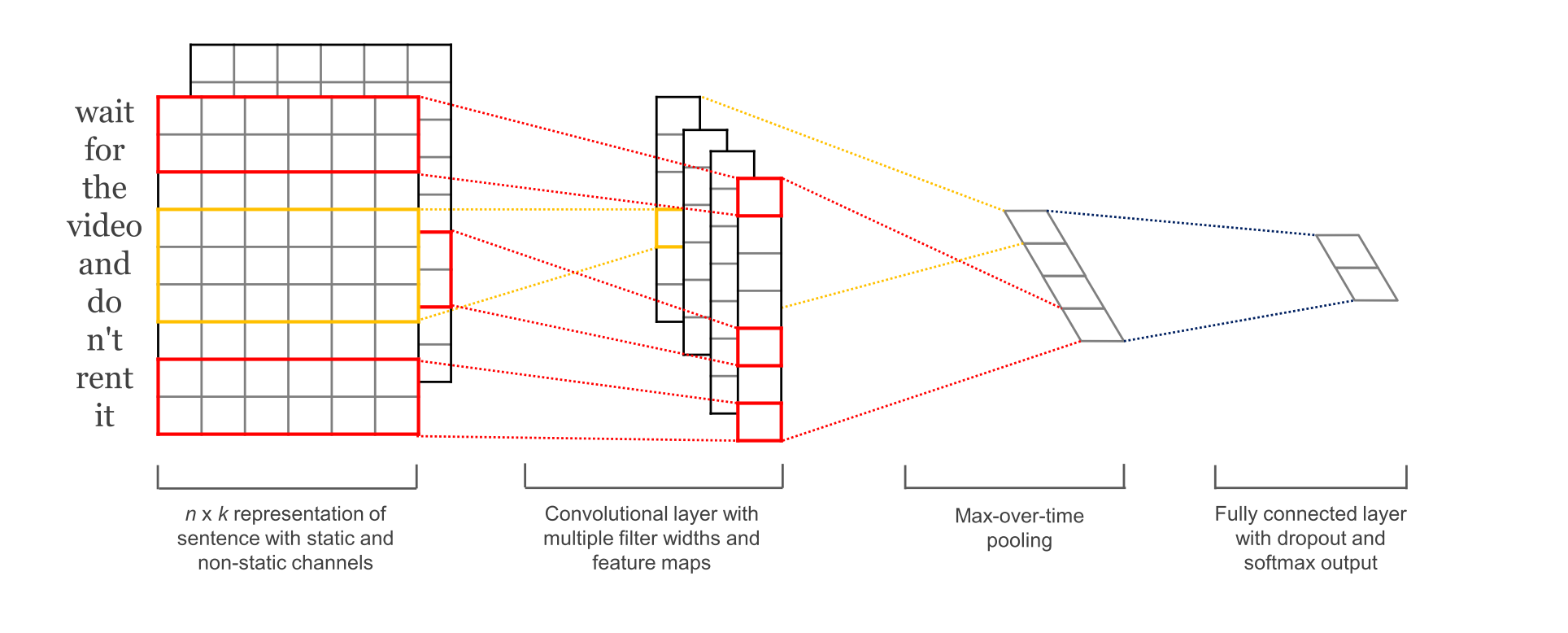
The first layers embeds words into low-dimensional vectors. The next layer performs convolutions over the embedded word vectors using multiple filter sizes. For example, sliding over 3, 4 or 5 words at a time. Next, we max-pool the result of the convolutional layer into a long feature vector, add dropout regularization, and classify the result using a softmax layer.

Because this is an educational post I decided to simplify the model from the original paper a little:

• We will not used pre-trained word2vec vectors for our word embeddings. Instead, we learn embeddings from scratch.
• We will not enforce L2 norm constraints on the weight vectors. A Sensitivity Analysis of (and Practitioners’ Guide to) Convolutional Neural Networks for Sentence Classification found that the constraints had little effect on the end result.
• The original paper experiments with two input data channels – static and non-static word vectors. We use only one channel.

It is relatively straightforward (a few dozen lines of code) to add the above extensions to the code here. Take a look at the exercises at the end of the post.

Implementation #

To allow various hyperparameter configurations we put our code into a TextCNN class, generating the model graph in the init function.

import tensorflow as tf
import numpy as np

class TextCNN(object):
    """
    A CNN for text classification.
    Uses an embedding layer, followed by a convolutional, max-pooling and softmax layer.
    """
    def __init__(
      self, sequence_length, num_classes, vocab_size,
      embedding_size, filter_sizes, num_filters):
        # Implementation...

To instantiate the class we then pass the following arguments:

• sequence_length – The length of our sentences. Remember that we padded all our sentences to have the same length (59 for our data set).
• num_classes – Number of classes in the output layer, two in our case (positive and negative).
• vocab_size – The size of our vocabulary. This is needed to define the size of our embedding layer, which will have shape [vocabulary_size, embedding_size].
• embedding_size – The dimensionality of our embeddings.
• filter_sizes – The number of words we want our convolutional filters to cover. We will have num_filters for each size specified here. For example, [3, 4, 5] means that we will have filters that slide over 3, 4 and 5 words respectively, for a total of 3 * num_filters filters.
• num_filters – The number of filters per filter size (see above).

Input Placeholders #

We start by defining the input data that we pass to our network:

# Placeholders for input, output and dropout
self.input_x = tf.placeholder(tf.int32, [None, sequence_length], name="input_x")
self.input_y = tf.placeholder(tf.float32, [None, num_classes], name="input_y")
self.dropout_keep_prob = tf.placeholder(tf.float32, name="dropout_keep_prob")

tf.placeholder creates a placeholder variable that we feed to the network when we execute it at train or test time. The second argument is the shape of the input tensor. None means that the length of that dimension could be anything. In our case, the first dimension is the batch size, and using None allows the network to handle arbitrarily sized batches.

The probability of keeping a neuron in the dropout layer is also an input to the network because we enable dropout only during training. We disable it when evaluating the model, but more on that later.

Embedding Layer #

The first layer we define is the embedding layer, which maps vocabulary word indices into low-dimensional vector representations. It’s essentially a lookup table that we learn from data.

with tf.device('/cpu:0'), tf.name_scope("embedding"):
    W = tf.Variable(
        tf.random_uniform([vocab_size, embedding_size], -1.0, 1.0),
        name="W")
    self.embedded_chars = tf.nn.embedding_lookup(W, self.input_x)
    self.embedded_chars_expanded = tf.expand_dims(self.embedded_chars, -1)

We’re using a couple of new features here so let’s go over them:

• tf.device("/cpu:0") forces an operation to be executed on the CPU. By default TensorFlow will try to put the operation on the GPU if one is available, but the embedding implementation doesn’t currently have GPU support and throws an error if placed on the GPU.
• tf.name_scope creates a new Name Scope with the name “embedding”. The scope adds all operations into a top-level node called “embedding” so that you get a nice hierarchy when visualizing your network in TensorBoard.

W is our embedding matrix that we learn during training. We initialize it using a random uniform distribution. tf.nn.embedding_lookup creates the actual embedding operation. The result of the embedding operation is a 3-dimensional tensor of shape [None, sequence_length, embedding_size].

TensorFlow’s convolutional conv2d operation expects a 4-dimensional tensor with dimensions corresponding to batch, width, height and channel. The result of our embedding doesn’t contain the channel dimension, so we add it manually, leaving us with a layer of shape [None, sequence_length, embedding_size, 1].

Convolution and Max-Pooling Layers #

Now we’re ready to build our convolutional layers followed by max-pooling. Remember that we use filters of different sizes. Because each convolution produces tensors of different shapes we need to iterate through them, create a layer for each of them, and then merge the results into one big feature vector.

pooled_outputs = []
for i, filter_size in enumerate(filter_sizes):
    with tf.name_scope("conv-maxpool-%s" % filter_size):
        # Convolution Layer
        filter_shape = [filter_size, embedding_size, 1, num_filters]
        W = tf.Variable(tf.truncated_normal(filter_shape, stddev=0.1), name="W")
        b = tf.Variable(tf.constant(0.1, shape=[num_filters]), name="b")
        conv = tf.nn.conv2d(
            self.embedded_chars_expanded,
            W,
            strides=[1, 1, 1, 1],
            padding="VALID",
            name="conv")
        # Apply nonlinearity
        h = tf.nn.relu(tf.nn.bias_add(conv, b), name="relu")
        # Max-pooling over the outputs
        pooled = tf.nn.max_pool(
            h,
            ksize=[1, sequence_length - filter_size + 1, 1, 1],
            strides=[1, 1, 1, 1],
            padding='VALID',
            name="pool")
        pooled_outputs.append(pooled)

# Combine all the pooled features
num_filters_total = num_filters * len(filter_sizes)
self.h_pool = tf.concat(3, pooled_outputs)
self.h_pool_flat = tf.reshape(self.h_pool, [-1, num_filters_total])

Here, W is our filter matrix and h is the result of applying the nonlinearity to the convolution output. Each filter slides over the whole embedding, but varies in how many words it covers. "VALID" padding means that we slide the filter over our sentence without padding the edges, performing a narrow convolution that gives us an output of shape [1, sequence_length - filter_size + 1, 1, 1]. Performing max-pooling over the output of a specific filter size leaves us with a tensor of shape [batch_size, 1, 1, num_filters]. This is essentially a feature vector, where the last dimension corresponds to our features. Once we have all the pooled output tensors from each filter size we combine them into one long feature vector of shape [batch_size, num_filters_total]. Using -1 in tf.reshape tells TensorFlow to flatten the dimension when possible.

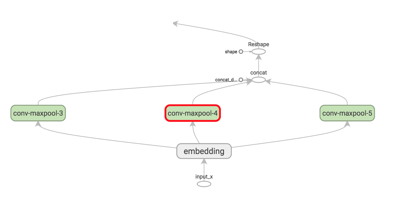
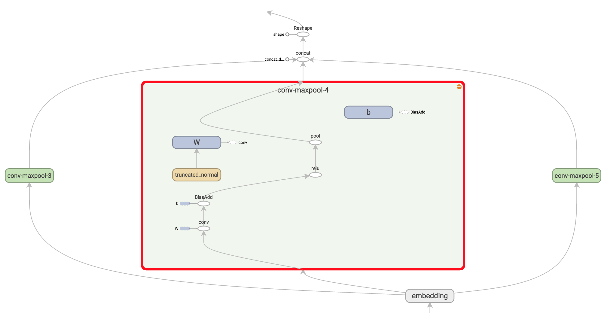
Take some time and try to understand the output shapes for each of these operations. You can also refer back to Understanding Convolutional Neural Networks for NLP to get some intuition. Visualizing the operations in TensorBoard may help as well (for specific filter sizes 3, 4 and 5 here):

Dropout Layer #

Dropout is the perhaps most popular method to regularize convolutional neural networks. A dropout layer stochastically “disables” a fraction of its neurons. This prevent neurons from co-adapting and forces them to learn individually useful features. The fraction of neurons we keep enabled is defined by the dropout_keep_prob input to our network. We set this to something like 0.5 during training, and to 1 (disable dropout) during evaluation.

# Add dropout
with tf.name_scope("dropout"):
    self.h_drop = tf.nn.dropout(self.h_pool_flat, self.dropout_keep_prob)

Scores and Predictions #

Using the feature vector from max-pooling (with dropout applied) we can generate predictions by doing a matrix multiplication and picking the class with the highest score. We could also apply a softmax function to convert raw scores into normalized probabilities, but that wouldn’t change our final predictions.

with tf.name_scope("output"):
    W = tf.Variable(tf.truncated_normal([num_filters_total, num_classes], stddev=0.1), name="W")
    b = tf.Variable(tf.constant(0.1, shape=[num_classes]), name="b")
    self.scores = tf.nn.xw_plus_b(self.h_drop, W, b, name="scores")
    self.predictions = tf.argmax(self.scores, 1, name="predictions")

Here, tf.nn.xw_plus_b is a convenience wrapper to perform the \(Wx + b\) matrix multiplication.

Loss and Accuracy #

Using our scores we can define the loss function. The loss is a measurement of the error our network makes, and our goal is to minimize it. The standard loss function for categorization problems it the cross-entropy loss.

# Calculate mean cross-entropy loss
with tf.name_scope("loss"):
    losses = tf.nn.softmax_cross_entropy_with_logits(self.scores, self.input_y)
    self.loss = tf.reduce_mean(losses)

Here, tf.nn.softmax_cross_entropy_with_logits is a convenience function that calculates the cross-entropy loss for each class, given our scores and the correct input labels. We then take the mean of the losses. We could also use the sum, but that makes it harder to compare the loss across different batch sizes and train/dev data.

We also define an expression for the accuracy, which is a useful quantity to keep track of during training and testing.

# Calculate Accuracy
with tf.name_scope("accuracy"):
    correct_predictions = tf.equal(self.predictions, tf.argmax(self.input_y, 1))
    self.accuracy = tf.reduce_mean(tf.cast(correct_predictions, "float"), name="accuracy")

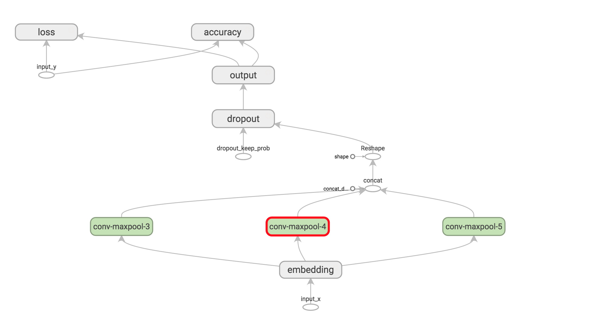
Visualizing the network #

That’s it, we’re done with our network definition. The full code network definition code is available here. To get the big picture we can also visualize the network in TensorBoard:

Training Procedure #

Before we define the training procedure for our network we need to understand some basics about how TensorFlow uses Sessions and Graphs. If you’re already familiar with these concepts feel free to skip this section.

In TensorFlow, a Session is the environment you are executing graph operations in, and it contains state about Variables and queues. Each session operates on a single graph. If you don’t explicitly use a session when creating variables and operations you are using the current default session created by TensorFlow. You can change the default session by executing commands within a session.as_default() block (see below).

A Graph contains operations and tensors. You can use multiple graphs in your program, but most programs only need a single graph. You can use the same graph in multiple sessions, but not multiple graphs in one session. TensorFlow always creates a default graph, but you may also create a graph manually and set it as the new default, like we do below. Explicitly creating sessions and graphs ensures that resources are released properly when you no longer need them.

with tf.Graph().as_default():
    session_conf = tf.ConfigProto(
      allow_soft_placement=FLAGS.allow_soft_placement,
      log_device_placement=FLAGS.log_device_placement)
    sess = tf.Session(config=session_conf)
    with sess.as_default():
        # Code that operates on the default graph and session comes here...

The allow_soft_placement setting allows TensorFlow to fall back on a device with a certain operation implemented when the preferred device doesn’t exist. For example, if our code places an operation on a GPU and we run the code on a machine without GPU, not using allow_soft_placement would result in an error. If log_device_placement is set, TensorFlow log on which devices (CPU or GPU) it places operations. That’s useful for debugging. FLAGS are command-line arguments to our program.

Instantiating the CNN and minimizing the loss #

When we instantiate our TextCNN models all the variables and operations defined will be placed into the default graph and session we’ve created above.

cnn = TextCNN(
    sequence_length=x_train.shape[1],
    num_classes=2,
    vocab_size=len(vocabulary),
    embedding_size=FLAGS.embedding_dim,
    filter_sizes=map(int, FLAGS.filter_sizes.split(",")),
    num_filters=FLAGS.num_filters)

Next, we define how to optimize our network’s loss function. TensorFlow has several built-in optimizers. We’re using the Adam optimizer.

global_step = tf.Variable(0, name="global_step", trainable=False)
optimizer = tf.train.AdamOptimizer(1e-4)
grads_and_vars = optimizer.compute_gradients(cnn.loss)
train_op = optimizer.apply_gradients(grads_and_vars, global_step=global_step)

train_op is a newly created operation that we can run to perform a gradient update on our parameters. Each execution of train_op is a training step. TensorFlow automatically figures out which variables are “trainable” and calculates their gradients. By defining a global_step variable and passing it to the optimizer we allow TensorFlow handle the counting of training steps for us. The global step will be automatically incremented by one every time you execute train_op.

Summaries #

TensorFlow has a concept of a summaries, which allow you to keep track of and visualize various quantities during training and evaluation. For example, you probably want to keep track of how your loss and accuracy evolve over time. You can also keep track of more complex quantities, such as histograms of layer activations. Summaries are serialized objects, and they are written to disk using a SummaryWriter.

# Output directory for models and summaries
timestamp = str(int(time.time()))
out_dir = os.path.abspath(os.path.join(os.path.curdir, "runs", timestamp))
print("Writing to {}\n".format(out_dir))

# Summaries for loss and accuracy
loss_summary = tf.scalar_summary("loss", cnn.loss)
acc_summary = tf.scalar_summary("accuracy", cnn.accuracy)

# Train Summaries
train_summary_op = tf.merge_summary([loss_summary, acc_summary])
train_summary_dir = os.path.join(out_dir, "summaries", "train")
train_summary_writer = tf.train.SummaryWriter(train_summary_dir, sess.graph_def)

# Dev summaries
dev_summary_op = tf.merge_summary([loss_summary, acc_summary])
dev_summary_dir = os.path.join(out_dir, "summaries", "dev")
dev_summary_writer = tf.train.SummaryWriter(dev_summary_dir, sess.graph_def)

We are separately keeping track of summaries for training and evaluation. In our case these are the same quantities, but you may have quantities that you want to track during training only, like parameter update values. tf.merge_summary is a convenience function that merges multiple summary operations into a single operation that we can execute.

Checkpointing #

Another TensorFlow feature you typically want to use is checkpointing – saving the parameters of your model to restore them later on. Checkpoints can be used to continue training at a later point, or to pick the best parameters setting using early stopping. Checkpoints are created using a Saver object.

# Checkpointing
checkpoint_dir = os.path.abspath(os.path.join(out_dir, "checkpoints"))
checkpoint_prefix = os.path.join(checkpoint_dir, "model")
# Tensorflow assumes this directory already exists so we need to create it
if not os.path.exists(checkpoint_dir):
    os.makedirs(checkpoint_dir)
saver = tf.train.Saver(tf.all_variables())

Initializing the variables #

Before we can train our model we also need to initialize the variables in our graph.

sess.run(tf.initialize_all_variables())

The initialize_all_variables function is a convenience function run all of the initializers we’ve defined for our variables. You can also call the initializer of your variables manually. That’s useful if you want to initialize your embeddings with pre-trained values for example.

Defining a single training step #

Let’s now define a function for a single training step, evaluating the model on a batch of data and updating the model parameters.

def train_step(x_batch, y_batch):
    """
    A single training step
    """
    feed_dict = {
      cnn.input_x: x_batch,
      cnn.input_y: y_batch,
      cnn.dropout_keep_prob: FLAGS.dropout_keep_prob
    }
    _, step, summaries, loss, accuracy = sess.run(
        [train_op, global_step, train_summary_op, cnn.loss, cnn.accuracy],
        feed_dict)
    time_str = datetime.datetime.now().isoformat()
    print("{}: step {}, loss {:g}, acc {:g}".format(time_str, step, loss, accuracy))
    train_summary_writer.add_summary(summaries, step)

feed_dict contains the data for the placeholder nodes we pass to our network. You must feed values for all placeholder nodes, or TensorFlow will throw an error. Another way to work with input data is using queues, but that’s beyond the scope of this post.

Next, we execute our train_op using session.run, which returns values for all the operations we ask it to evaluate. Note that train_op returns nothing, it just updates the parameters of our network. Finally, we print the loss and accuracy of the current training batch and save the summaries to disk. Note that the loss and accuracy for a training batch may vary significantly across batches if your batch size is small. And because we’re using dropout your training metrics may start out being worse than your evaluation metrics.

We write a similar function to evaluate the loss and accuracy on an arbitrary data set, such as a validation set or the whole training set. Essentially this function does the same as the above, but without the training operation. It also disables dropout.

def dev_step(x_batch, y_batch, writer=None):
    """
    Evaluates model on a dev set
    """
    feed_dict = {
      cnn.input_x: x_batch,
      cnn.input_y: y_batch,
      cnn.dropout_keep_prob: 1.0
    }
    step, summaries, loss, accuracy = sess.run(
        [global_step, dev_summary_op, cnn.loss, cnn.accuracy],
        feed_dict)
    time_str = datetime.datetime.now().isoformat()
    print("{}: step {}, loss {:g}, acc {:g}".format(time_str, step, loss, accuracy))
    if writer:
        writer.add_summary(summaries, step)

Training loop #

Finally, we’re ready to write our training loop. We iterate over batches of our data, call the train_step function for each batch, and occasionally evaluate and checkpoint our model:

# Generate batches
batches = data_helpers.batch_iter(
    zip(x_train, y_train), FLAGS.batch_size, FLAGS.num_epochs)
# Training loop. For each batch...
for batch in batches:
    x_batch, y_batch = zip(*batch)
    train_step(x_batch, y_batch)
    current_step = tf.train.global_step(sess, global_step)
    if current_step % FLAGS.evaluate_every == 0:
        print("\nEvaluation:")
        dev_step(x_dev, y_dev, writer=dev_summary_writer)
        print("")
    if current_step % FLAGS.checkpoint_every == 0:
        path = saver.save(sess, checkpoint_prefix, global_step=current_step)
        print("Saved model checkpoint to {}\n".format(path))

Here, batch_iter is a helper function I wrote to batch the data, and tf.train.global_step is convenience function that returns the value of global_step. The full code for training is also available here.

Visualizing Results in TensorBoard #

Our training script writes summaries to an output directory, and by pointing TensorBoard to that directory we can visualize the graph and the summaries we created.

tensorboard --logdir /PATH_TO_CODE/runs/1449760558/summaries/

Running the training procedure with default parameters (128-dimensional embeddings, filter sizes of 3, 4 and 5, dropout of 0.5 and 128 filters per filter size) results in the following loss and accuracy plots (blue is training data, red is 10% dev data).

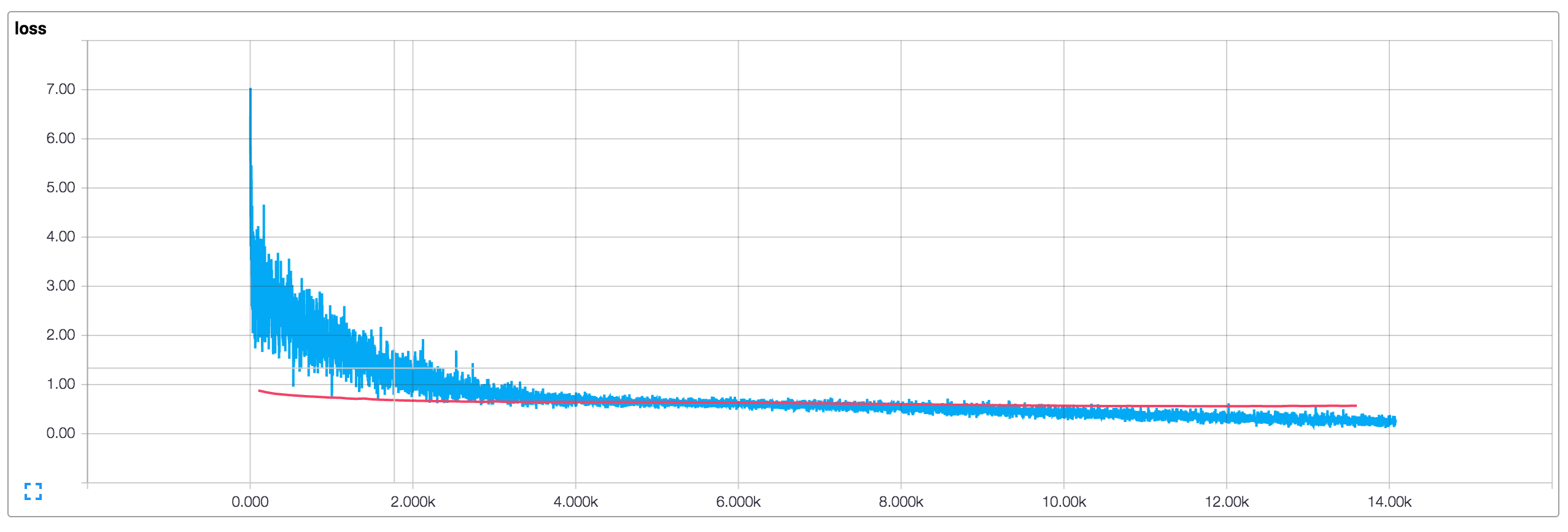
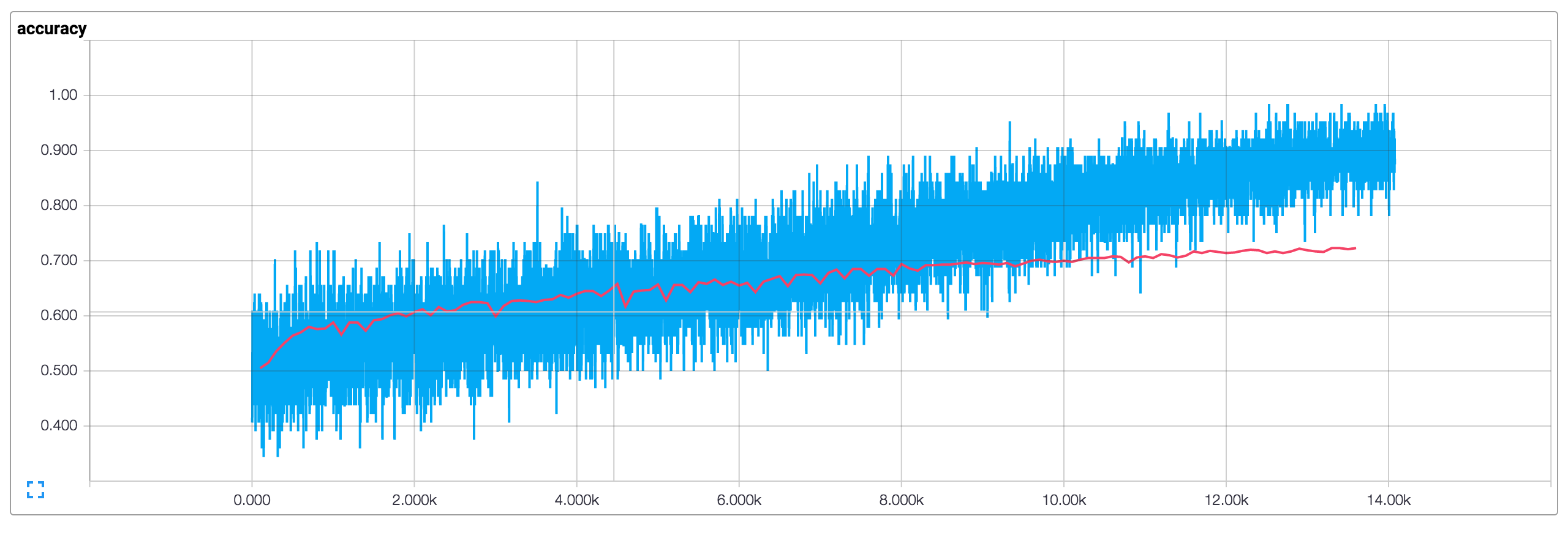
There are a couple of things that stand out:

• Our training metrics are not smooth because we use small batch sizes. If we used larger batches (or evaluated on the whole training set) we would get a smoother blue line.
• Because dev accuracy is significantly below training accuracy it seems like our network is overfitting the training data, suggesting that we need more data (the MR dataset is very small), stronger regularization, or fewer model parameters. For example, I experimented with adding additional L2 penalties for the weights at the last layer and was able to bump up the accuracy to 76%, close to that reported in the original paper.
• The training loss and accuracy starts out significantly below the dev metrics due to dropout applied to it.

You can play around with the code and try running the model with various parameter configuration. Code and instructions are available on Github.

Extensions and Exercises #

Here are a couple of useful exercises that may improve the performance of the model:

• Initialize the embeddings with pre-trained word2vec vectors. To make this work you need to use 300-dimensional embeddings and initialize them with the pre-trained values.
• Constrain the L2 norm of the weight vectors in the last layer, just like the original paper. You can do this by defining a new operation that updates the weight values after each training step.
• Add L2 regularization to the network to combat overfitting, also experiment with increasing the dropout rate. (The code on Github already includes L2 regularization, but it is disabled by default)
• Add histogram summaries for weight updates and layer actions and visualize them in TensorBoard.