Recurrent Neural Networks Tutorial, Part 3 – Backpropagation Through Time and Vanishing Gradients

This the third part of the Recurrent Neural Network Tutorial.

In the previous part of the tutorial we implemented a RNN from scratch, but didn’t go into detail on how Backpropagation Through Time (BPTT) algorithms calculates the gradients. In this part we’ll give a brief overview of BPTT and explain how it differs from traditional backpropagation. We will then try to understand the vanishing gradient problem, which has led to the development of LSTMs and GRUs, two of the currently most popular and powerful models used in NLP (and other areas). The vanishing gradient problem was originally discovered by Sepp Hochreiter in 1991 and has been receiving attention again recently due to the increased application of deep architectures.

To fully understand this part of the tutorial I recommend being familiar with how partial differentiation and basic backpropagation works. If you are not, you can find excellent tutorials here and here and here, in order of increasing difficulty.

Backpropagation Through Time (BPTT) #

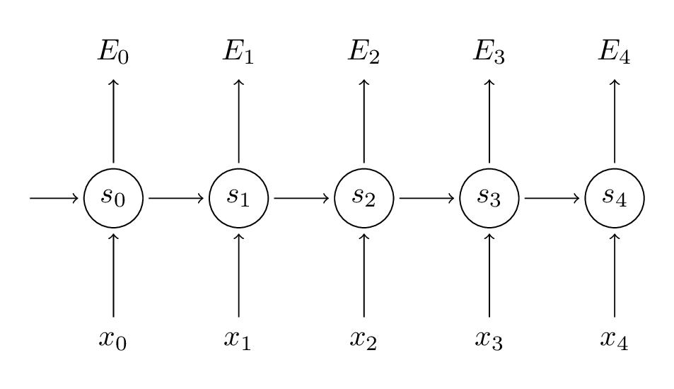
Let’s quickly recap the basic equations of our RNN. Note that there’s a slight change in notation from $o$ to $\hat{y}$. That’s only to stay consistent with some of the literature out there that I am referencing.

$$ \begin{aligned} s_t &= \tanh(Ux_t + Ws_{t-1}) \\ \hat{y}_t &= \mathrm{softmax}(Vs_t) \end{aligned} $$

We also defined our loss, or error, to be the cross entropy loss, given by:

$$ \begin{aligned} E_t(y_t, \hat{y}_t) &= - y_t \log \hat{y}_t \\ E(y, \hat{y}) &=\sum\limits_t E_t(y_t,\hat{y}_t) \\ &= -\sum\limits_t y_t \log \hat{y}_t \\ \end{aligned} $$

Here, $y_t$ is the correct word at time step $t$, and $\hat{y}_t$ is our prediction. We typically treat the full sequence (sentence) as one training example, so the total error is just the sum of the errors at each time step (word).

Remember that our goal is to calculate the gradients of the error with respect to our parameters $U, V$ and $W$ and then learn good parameters using Stochastic Gradient Descent. Just like we sum up the errors, we also sum up the gradients at each time step for one training example: $\frac{\partial E}{\partial W} = \sum\limits_t \frac{\partial E_t}{\partial W}$.

To calculate these gradients we use the chain rule of differentiation. That’s the backpropagation algorithm when applied backwards starting from the error. For the rest of this post we’ll use $E_3$ as an example, just to have concrete numbers to work with.

$$ \begin{aligned} \frac{\partial E_3}{\partial V} &=\frac{\partial E_3}{\partial \hat{y}_3}\frac{\partial\hat{y}_3}{\partial V}\\ &=\frac{\partial E_3}{\partial \hat{y}_3}\frac{\partial\hat{y}_3}{\partial z_3}\frac{\partial z_3}{\partial V}\\ &=(\hat{y}_3 - y_3) \otimes s_3 \\ \end{aligned} $$

In the above, $z_3 =Vs_3$, and $\otimes $ is the outer product of two vectors. Don’t worry if you don’t follow the above, I skipped several steps and you can try calculating these derivatives yourself (good exercise!). The point I’m trying to get across is that $\frac{\partial E_3}{\partial V} $ only depends on the values at the current time step, $\hat{y}_3, y_3, s_3 $. If you have these, calculating the gradient for $V$ a simple matrix multiplication.

But the story is different for $\frac{\partial E_3}{\partial W}$ (and for $U$). To see why, we write out the chain rule, just as above:

$$ \begin{aligned} \frac{\partial E_3}{\partial W} &= \frac{\partial E_3}{\partial \hat{y}_3}\frac{\partial\hat{y}_3}{\partial s_3}\frac{\partial s_3}{\partial W}\\ \end{aligned} $$

Now, note that $s_3 = \tanh(Ux_t + Ws_2)$ depends on $s_2$, which depends on $W$ and $s_1$, and so on. So if we take the derivative with respect to $W$ we can’t simply treat $s_2$ as a constant! We need to apply the chain rule again and what we really have is this:

$$ \begin{aligned} \frac{\partial E_3}{\partial W} &= \sum\limits_{k=0}^{3} \frac{\partial E_3}{\partial \hat{y}_3}\frac{\partial\hat{y}_3}{\partial s_3}\frac{\partial s_3}{\partial s_k}\frac{\partial s_k}{\partial W}\\ \end{aligned} $$

We sum up the contributions of each time step to the gradient. In other words, because $W$ is used in every step up to the output we care about, we need to backpropagate gradients from $t=3$ through the network all the way to $t=0$:

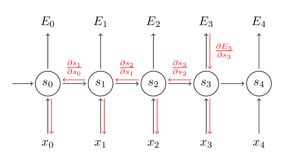
Unrolled Recurrent Neural Network for 5 time steps with gradients

Note that this is exactly the same as the standard backpropagation algorithm that we use in deep Feedforward Neural Networks. The key difference is that we sum up the gradients for $W$ at each time step. In a traditional NN we don’t share parameters across layers, so we don’t need to sum anything. But this also means that BPTT is just a fancy name for standard backpropagation on an unrolled RNN. Just like with Backpropagation you could define a delta vector that you pass backwards, e.g.: $\delta_2^{(3)} = \frac{\partial E_3}{\partial z_2} =\frac{\partial E_3}{\partial s_3}\frac{\partial s_3}{\partial s_2}\frac{\partial s_2}{\partial z_2}$ with $z_2 = Ux_2+ Ws_1$. Then the same equations will apply.

In code, a naive implementation of BPTT looks something like this:

def bptt(self, x, y):
    T = len(y)
    # Perform forward propagation
    o, s = self.forward_propagation(x)
    # We accumulate the gradients in these variables
    dLdU = np.zeros(self.U.shape)
    dLdV = np.zeros(self.V.shape)
    dLdW = np.zeros(self.W.shape)
    delta_o = o
    delta_o[np.arange(len(y)), y] -= 1.
    # For each output backwards...
    for t in np.arange(T)[::-1]:
        dLdV += np.outer(delta_o[t], s[t].T)
        # Initial delta calculation: dL/dz
        delta_t = self.V.T.dot(delta_o[t]) * (1 - (s[t] ** 2))
        # Backpropagation through time (for at most self.bptt_truncate steps)
        for bptt_step in np.arange(max(0, t-self.bptt_truncate), t+1)[::-1]:
            # print "Backpropagation step t=%d bptt step=%d " % (t, bptt_step)
            # Add to gradients at each previous step
            dLdW += np.outer(delta_t, s[bptt_step-1])              
            dLdU[:,x[bptt_step]] += delta_t
            # Update delta for next step dL/dz at t-1
            delta_t = self.W.T.dot(delta_t) * (1 - s[bptt_step-1] ** 2)
    return [dLdU, dLdV, dLdW]

This should also give you an idea of why standard RNNs are hard to train: Sequences (sentences) can be quite long, perhaps 20 words or more, and thus you need to back-propagate through many layers. In practice many people truncate the backpropagation to a few steps.

The Vanishing Gradient Problem #

In previous parts of the tutorial I mentioned that RNNs have difficulties learning long-range dependencies – interactions between words that are several steps apart. That’s problematic because the meaning of an English sentence is often determined by words that aren’t very close: “The man who wore a wig on his head went inside”. The sentence is really about a man going inside, not about the wig. But it’s unlikely that a plain RNN would be able capture such information. To understand why, let’s take a closer look at the gradient we calculated above:

Note that $\frac{\partial s_3}{\partial s_k} $ is a chain rule in itself! For example, $\frac{\partial s_3}{\partial s_1} =\frac{\partial s_3}{\partial s_2}\frac{\partial s_2}{\partial s_1}$. Also note that because we are taking the derivative of a vector function with respect to a vector, the result is a matrix (called the Jacobian matrix) whose elements are all the pointwise derivatives. We can rewrite the above $\frac{\partial s_3}{\partial s_k} $:

$$ \left(\prod_{j=k+1}^3\frac{\partial s_j}{\partial s_{j-1}}\right) \frac{\partial s_k}{\partial W} $$

It turns out (I won’t prove it here but this paper goes into detail) that the 2-norm, which you can think of it as an absolute value, of the above Jacobian matrix has an upper bound of 1. This makes intuitive sense because our $tanh$ (or sigmoid) activation function maps all values into a range between -1 and 1, and the derivative is bounded by 1 (1/4 in the case of sigmoid) as well:

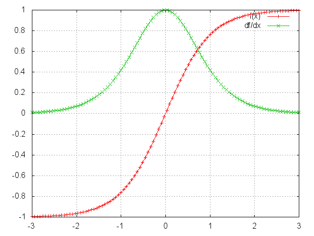
You can see that the $\tanh$ and sigmoid functions have derivatives of 0 at both ends. They approach a flat line. When this happens we say the corresponding neurons are saturated. They have a zero gradient and drive other gradients in previous layers towards 0. Thus, with small values in the matrix and multiple matrix multiplications ($t-k$ in particular) the gradient values are shrinking exponentially fast, eventually vanishing completely after a few time steps. Gradient contributions from “far away” steps become zero, and the state at those steps doesn’t contribute to what you are learning: You end up not learning long-range dependencies. Vanishing gradients aren’t exclusive to RNNs. They also happen in deep Feedforward Neural Networks. It’s just that RNNs tend to be very deep (as deep as the sentence length in our case), which makes the problem common.

It is easy to imagine that, depending on our activation functions and network parameters, we could get exploding instead of vanishing gradients if the values of the Jacobian matrix are large. Indeed, that’s called the exploding gradient problem. The reason that vanishing gradients have received more attention than exploding gradients is two-fold. For one, exploding gradients are obvious. Your gradients will become NaN (not a number) and your program will crash. Secondly, clipping the gradients at a pre-defined threshold (as discussed in this paper) is a simple and effective solution to exploding gradients. Vanishing gradients are more problematic because it’s not obvious when they occur or how to deal with them.

Fortunately, there are a few ways to combat the vanishing gradient problem. Proper initialization of the $W$ matrix can reduce the effect of vanishing gradients. So can regularization. A more preferred solution is to use ReLU instead of $tanh$ or sigmoid activation functions. The ReLU derivative is a constant of either 0 or 1, so it isn’t as likely to suffer from vanishing gradients. An even more popular solution is to use Long Short-Term Memory (LSTM) or Gated Recurrent Unit (GRU) architectures. LSTMs were first proposed in 1997 and are the perhaps most widely used models in NLP today. GRUs, first proposed in 2014, are simplified versions of LSTMs. Both of these RNN architectures were explicitly designed to deal with vanishing gradients and efficiently learn long-range dependencies. We’ll cover them in the next part of this tutorial.