Speeding up your Neural Network with Theano and the GPU
The full code is available as an Jupyter Notebook on Github!
In a previous blog post we build a simple Neural Network from scratch. Let’s build on top of this and speed up our code using the Theano library. With Theano we can make our code not only faster, but also more concise!
What is Theano? #
Theano describes itself as a Python library that lets you to define, optimize, and evaluate mathematical expressions, especially ones with multi-dimensional arrays. The way I understand Theano is that it allows me to define graphs of computations. Under the hood Theano optimizes these computations in a variety of ways, including avoiding redundant calculations, generating optimized C code, and (optionally) using the GPU. Theano also has the capability to automatically differentiate mathematical expressions. By modeling computations as graphs it can calculate complex gradients using the chain rule. This means we no longer need to compute the gradients ourselves!
Because Neural Networks are easily expressed as graphs of computations, Theano is a great fit. It’s probably the main use case and Theano includes several convenience functions for neural networks.
The Setup #
The setup is identical to that in Implementing a Neural Network from Scratch, which I recommend you read (or at least skim) first. I’ll just quickly recap: We have two classes (red and blue) and want to train a Neural Network classifier that separates the two. We will train a 3-layer Neural Network, with input layer size 2, output layer size 2, and hidden layer size 3. We will use batch gradient descent with a fixed learning rate to train our network.

Defining the Computation Graph in Theano #
The first thing we need to is define our computations using Theano. We start by defining our input data matrix X and our training labels y:
import theano
import theano.tensor as T

# Our data vectors
X = T.matrix('X') # matrix of doubles
y = T.lvector('y') # vector of int64
The crucial thing to understand: We have not assigned any values to X or y. All we have done is defined mathematical expressions for them. We can use these expressions in subsequent calculations. If we want to evaluate an expression we can call its eval method. For example, to evaluate the expression X * 2 for a given value of X we could do the following:
(X * 2).eval({X : [[1,1],[2,2]] })
Theano handles the type checking for us, which is very useful when defining more complex expressions. Trying to assign a value of the wrong data type to X would result in an error. Here is the full list of Theano types.
X and y above are stateless. Whenever we want to evaluate an expression that depends on them we need to provide their values. Theano also has something called shared variables, which have internal state associated with them. Their value is kept in memory and can be shared by all functions that use them. Shared variables can also be updated, and Theano includes low-level optimizations that makes updating them very efficient, especially on GPUs. Our network parameters \(W_1, b_1, W_2, b_2\) are constantly updated using gradient descent, so they are perfect candidates for shared variables:
# Shared variables with initial values. We need to learn these.
W1 = theano.shared(np.random.randn(nn_input_dim, nn_hdim), name='W1')
b1 = theano.shared(np.zeros(nn_hdim), name='b1')
W2 = theano.shared(np.random.randn(nn_hdim, nn_output_dim), name='W2')
b2 = theano.shared(np.zeros(nn_output_dim), name='b2')
Next, let’s define expressions for our forward propagation. The calculations are identical to what we did in our previous implementation, just that we are defining Theano expressions. Again, remember that these expressions are not evaluated, we are just defining them. You can think of them as lambda expressions that require input values when called. We also use some of Theano’s convenience functions like nnet.softmax and nnet.categorical_crossentropy to replace our manual implementations:
# Forward propagation
# Note: We are just defining the expressions, nothing is evaluated here!
z1 = X.dot(W1) + b1
a1 = T.tanh(z1)
z2 = a1.dot(W2) + b2
y_hat = T.nnet.softmax(z2) # output probabilties

# The regularization term (optional)
loss_reg = 1./num_examples * reg_lambda/2 * (T.sum(T.sqr(W1)) + T.sum(T.sqr(W2)))
# the loss function we want to optimize
loss = T.nnet.categorical_crossentropy(y_hat, y).mean() + loss_reg

# Returns a class prediction
prediction = T.argmax(y_hat, axis=1)
We saw how we can evaluate a Theano expression by calling its eval method. A much more convenient way is to create a Theano function for expressions we want to evaluate. To create a function we need to define its inputs and outputs. For example, to calculate the loss, we need to know the values for \(X\) and \(y\). Once created, we can call it function just like any other Python function.
# Theano functions that can be called from our Python code
forward_prop = theano.function([X], y_hat)
calculate_loss = theano.function([X, y], loss)
predict = theano.function([X], prediction)

# Example call: Forward Propagation
forward_prop([[1,2]])
Now is a good time to get a sense of how Theano constructs a computational graph. Looking at the expressions for \(\hat{y}\), we can see that it depends on \(z2\), which in turn depends on \(a_1\), \(W_2\) and \(b_2\), and so on. Theano lets us visualize this:
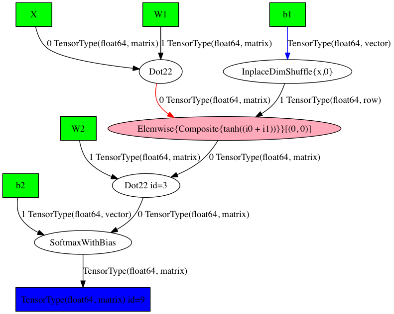
This is the optimized computational graph that Theano has constructed for our forward_prop function. We can also get a textual description:
SoftmaxWithBias \[@A\] ” 4
|Dot22 \[@B\] ” 3
| |Elemwise{Composite{tanh((i0 + i1))}}\[(0, 0)\] \[@C\] ” 2
| | |Dot22 \[@D\] ” 1
| | | |X \[@E\]
| | | |W1 \[@F\]
| | |InplaceDimShuffle{x,0} \[@G\] ” 0
| | |b1 \[@H\]
| |W2 \[@I\]
|b2 \[@J\]
What’s left is defining the updates to the network parameters we use with gradient descent. We previously calculated the gradients using backpropagation. We could express the same calculations using Theano (see code that’s commented out below), but it’s much easier if we let Theano calculate the derivatives for us! We need the derivates of our loss function \(L\) with respect to our parameters: \(\frac{\partial L}{\partial W_2}\), \(\frac{\partial L}{\partial b_2}\), \(\frac{\partial L}{\partial W_1}\), \(\frac{\partial L}{\partial b_1}\):
# Easy: Let Theano calculate the derivatives for us!
dW2 = T.grad(loss, W2)
db2 = T.grad(loss, b2)
dW1 = T.grad(loss, W1)
db1 = T.grad(loss, b1)

# Backpropagation (Manual)
# Note: We are just defining the expressions, nothing is evaluated here!
# y_onehot = T.eye(2)[y]
# delta3 = y_hat - y_onehot
# dW2 = (a1.T).dot(delta3) * (1. + reg_lambda)
# db2 = T.sum(delta3, axis=0)
# delta2 = delta3.dot(W2.T) * (1. - T.sqr(a1))
# dW1 = T.dot(X.T, delta2) * (1 + reg_lambda)
# db1 = T.sum(delta2, axis=0)
Because we defined \(W_2, b_2, W_1, b_1\) as shared variables we can use Theano’s update mechanism to update their values. The following function (without return value) does a single gradient descent update given \(X\) and \(y\) as inputs:
gradient_step = theano.function(
    [X, y],
    updates=((W2, W2 - epsilon * dW2),
             (W1, W1 - epsilon * dW1),
             (b2, b2 - epsilon * db2),
             (b1, b1 - epsilon * db1)))
Note that we don’t need to explicitly do a forward propagation here. Theano knows that our gradients depend on our predictions from the forward propagation and it will handle all the necessary calculations for us. It does everything it needs to update the values.
Let’s now define a function to train a Neural Network using gradient descent. Again, it’s equivalent to what we had in our original code, only that we are now calling the gradient_step function defined above instead of doing the calculations ourselves.
# This function learns parameters for the neural network and returns the model.
# - num_passes: Number of passes through the training data for gradient descent
# - print_loss: If True, print the loss every 1000 iterations
def build_model(num_passes=20000, print_loss=False):

    # Re-Initialize the parameters to random values. We need to learn these.
    # (Needed in case we call this function multiple times)
    np.random.seed(0)
    W1.set_value(np.random.randn(nn_input_dim, nn_hdim) / np.sqrt(nn_input_dim))
    b1.set_value(np.zeros(nn_hdim))
    W2.set_value(np.random.randn(nn_hdim, nn_output_dim) / np.sqrt(nn_hdim))
    b2.set_value(np.zeros(nn_output_dim))

    # Gradient descent. For each batch...
    for i in xrange(0, num_passes):
        # This will update our parameters W2, b2, W1 and b1!
        gradient_step(train_X, train_y)

        # Optionally print the loss.
        # This is expensive because it uses the whole dataset, so we don't want to do it too often.
        if print_loss and i % 1000 == 0:
            print "Loss after iteration %i: %f" %(i, calculate_loss(train_X, train_y))
# Build a model with a 3-dimensional hidden layer
build_model(print_loss=True)

# Plot the decision boundary
plot_decision_boundary(lambda x: predict(x))
plt.title("Decision Boundary for hidden layer size 3")
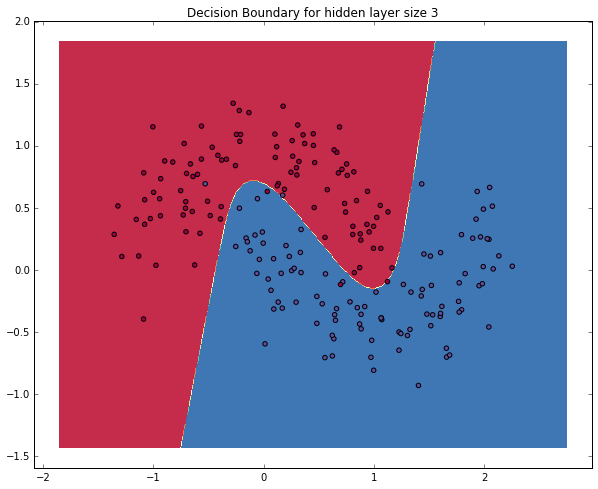
That’s it! We’ve just ported our code over to Theano. I got a 2-3x speedup on my Macbook (it would likely be more if we had larger matrix multiplications). Note that we’re not using a GPU yet. Let’s do that next!
Running on a GPU #
To speed things up further Theano can make use of your GPU. Theano relies on Nvidia’s CUDA platform, so yo need a CUDA-enabled graphics card. If you don’t have one (for example if you’re on a Macbook with an integrated GPU like me) you could spin up a GPU-optimized Amazon EC2 instance and try things there. To use the GPU with Theano you must have the CUDA toolkit installed and set a few environment variables. The repository readme contains instructions on how to setup CUDA on an EC2 isntance.
While any Theano code will run just fine with the GPU enabled you probably want to spend time optimizing your code get optimal performance. Running code that isn’t optimized for a GPU may actually be slower on a GPU than a CPU due to excessive data transfers.
Here are some things you must consider when writing Theano code for a GPU:
- The default floating point data type is
float64, but in order to use the GPU you must usefloat32. There are several ways to do this in Theano. You can either use the fulled typed tensor constructors likeT.fvectoror settheano.config.floatXtofloat32and use the simple tensor constructors likeT.vector. - Shared variables must be initialized with values of type
float32in order to be stored on the GPU. In other words, when creating a shared variable from a numpy array you must initialize the array with thedtype=float32argument, or cast it using theastypefunction. See the numpy data type documentation for more details. - Be very careful with data transfers to and from the GPU. Ideally you want all your data on the GPU. Ways to achieve this include initializing commonly used data as shared variables with a
float32data type, and to avoid copying return values back to the host using thegpu_from_hostfunction. Theano includes profiling capabilities that allow you to debug how much time you are spending on data transfers.
With all that in mind, let’s modify our code to run well on a GPU. I’ll highlight the most important changes we here, but the full code is available here or at the bottom of the post.
First, to see a significant speedup we should increase the size of our data so that the computation time will be dominated by matrix multiplication and other mathematical operations (as opposed to looping in Python code and assigning values).
train_X, train_y = sklearn.datasets.make_moons(5000, noise=0.20)
nn_hdim = 1000
Next, we change our scalar values to float32 to ensure that our calculations stay within that type. If we multiplied a float32 value by a float64 value the return value would be a float64.
epsilon = np.float32(0.01)
reg_lambda = np.float32(0.01)
To force the storage of our data on the GPU we use shared variables of type float32. Because we are constantly using the input data X and y to perform gradient updates we store those on the GPU as well:
# These float32 values will be initialized on the GPU
X = theano.shared(train_X.astype('float32'), name='X')
y = theano.shared(train_y_onehot.astype('float32'), name='y')
W1 = theano.shared(np.random.randn(nn_input_dim, nn_hdim).astype('float32'), name='W1')
b1 = theano.shared(np.zeros(nn_hdim).astype('float32'), name='b1')
W2 = theano.shared(np.random.randn(nn_hdim, nn_output_dim).astype('float32'), name='W2')
b2 = theano.shared(np.zeros(nn_output_dim).astype('float32'), name='b2')
We remove the inputs from our functions since the X and y values are stored as shared variables (on the GPU) now. We no longer need to pass them to the function calls.
gradient_step = theano.function(
    inputs=[],
    updates=((W2, W2 - epsilon * dW2),
             (W1, W1 - epsilon * dW1),
             (b2, b2 - epsilon * db2),
             (b1, b1 - epsilon * db1)))

# Does a gradient step and updates the values of our paremeters
gradient_step()
Running and Evaluation #
To use a GPU you must run the code with the THEANO_FLAGS=device=gpu,floatX=float32 environment variable set. I tested the GPU-optimized code on a g2.2xlarge AWS EC2 instance. Running one gradient_step() on the CPU took around 250ms. With the GPU enabled it merely took 7.5ms. That’s a 40x speedup, and if our dataset or parameter space were larger we would probably see an even more significant speedup.
Full GPU-optimzied code #
# Generate a dataset
np.random.seed(0)
train_X, train_y = sklearn.datasets.make_moons(5000, noise=0.20)
train_y_onehot = np.eye(2)[train_y]

# Size definitions
num_examples = len(train_X) # training set size
nn_input_dim = 2 # input layer dimensionality
nn_output_dim = 2 # output layer dimensionality
nn_hdim = 1000 # hiden layer dimensionality

# Gradient descent parameters (I picked these by hand)
epsilon = np.float32(0.01) # learning rate for gradient descent
reg_lambda = np.float32(0.01) # regularization strength

# GPU NOTE: Conversion to float32 to store them on the GPU!
X = theano.shared(train_X.astype('float32')) # initialized on the GPU
y = theano.shared(train_y_onehot.astype('float32'))

# GPU NOTE: Conversion to float32 to store them on the GPU!
W1 = theano.shared(np.random.randn(nn_input_dim, nn_hdim).astype('float32'), name='W1')
b1 = theano.shared(np.zeros(nn_hdim).astype('float32'), name='b1')
W2 = theano.shared(np.random.randn(nn_hdim, nn_output_dim).astype('float32'), name='W2')
b2 = theano.shared(np.zeros(nn_output_dim).astype('float32'), name='b2')

# Forward propagation
z1 = X.dot(W1) + b1
a1 = T.tanh(z1)
z2 = a1.dot(W2) + b2
y_hat = T.nnet.softmax(z2)

# The regularization term (optional)
loss_reg = 1./num_examples * reg_lambda/2 * (T.sum(T.sqr(W1)) + T.sum(T.sqr(W2)))
# the loss function we want to optimize
loss = T.nnet.categorical_crossentropy(y_hat, y).mean() + loss_reg
# Returns a class prediction
prediction = T.argmax(y_hat, axis=1)

# Gradients
dW2 = T.grad(loss, W2)
db2 = T.grad(loss, b2)
dW1 = T.grad(loss, W1)
db1 = T.grad(loss, b1)

# Note that we removed the input values because we will always use the same shared variable
# GPU NOTE: Removed the input values to avoid copying data to the GPU.
forward_prop = theano.function([], y_hat)
calculate_loss = theano.function([], loss)
predict = theano.function([], prediction)

# GPU NOTE: Removed the input values to avoid copying data to the GPU.
gradient_step = theano.function(
    [],
    # profile=True,
    updates=((W2, W2 - epsilon * dW2),
             (W1, W1 - epsilon * dW1),
             (b2, b2 - epsilon * db2),
             (b1, b1 - epsilon * db1)))

def build_model(num_passes=20000, print_loss=False):
    # Re-Initialize the parameters to random values. We need to learn these.
    np.random.seed(0)
    # GPU NOTE: Conversion to float32 to store them on the GPU!
    W1.set_value((np.random.randn(nn_input_dim, nn_hdim) / np.sqrt(nn_input_dim)).astype('float32'))
    b1.set_value(np.zeros(nn_hdim).astype('float32'))
    W2.set_value((np.random.randn(nn_hdim, nn_output_dim) / np.sqrt(nn_hdim)).astype('float32'))
    b2.set_value(np.zeros(nn_output_dim).astype('float32'))

    # Gradient descent. For each batch...
    for i in xrange(0, num_passes):
        # This will update our parameters W2, b2, W1 and b1!
        gradient_step()

        # Optionally print the loss.
        # This is expensive because it uses the whole dataset, so we don't want to do it too often.
        if print_loss and i % 1000 == 0:
            print "Loss after iteration %i: %f" %(i, calculate_loss())


# Profiling
# theano.config.profile = True
# theano.config.profile_memory = True
# gradient_step()
# theano.printing.debugprint(gradient_step)
# print gradient_step.profile.summary()

%timeit gradient_step()
The full code is available as an Jupyter Notebook on Github!